Hello,
In the Prof. Harris's text book  "Multirate Signal Processing for Communications" (pag. 62), a FIR filter to realize decimation (M=32, Stopband Atenutation = -60 dB) is used as example to show how to deal with sidelobe supression decrease from -60dB to -51.2 dB which is caused by the adjacent spectrum replicas after decimation.

The "integrated sidelobe level" (-36.1 dB) is mentioned and the new value for this sidelobe supression was named as "effective alias sidelobe supression".
Anyone know how to calculate these "integrated sidelobe level" and "effective alias sidelobe supression" values?

Text:
/*
The filter designed for 60-dB 'sidelobe levels is used in a 32-to-1 down sampling application. If the side-lobes are equiripple at 60-dB the integrated side-lobe level is -36.1-dB which, when distributed over the remaining bandwidth of 1/32 (-15.1-dB) of input sample rate, results in an effective alias side-lobe suppression of -51.2-dB, equivalent to a 9-dBloss.
*/

After that, the filter is re-designed with a higher stopband attenuation (to compensate the "effective" degradation when is decimated) and adapted to have 1/f slope stopband sidelobes.

Thank you

1012.3638.pdf

Hi jluqueq.

See attached is a file concerning calculating integrated sidelobe levels.

It is advanced.

Best I could do in my research for you.

convolver

I'm not sure of the exact shape of the concept that Dr. Harris is trying to get across, and I probably can't without reading the book.  However, it appears that his general notion is that when down-sampling may not give you as much attenuation as you would think at first blush, and that you should take this into account in designing your filters.

I suspect that what he's saying is that after filtering and before decimation, the signal is going to have components that are well away from the desired signal -- but after decimation, thanks to aliasing, those components will be in the side band of the newly-decimated signal.

Again, working on suspicion, I would suggest that you construct a received signal that consists of a pure tone at the center of your desired signal band, and white noise everywhere else.  If I'm reading your snippet of his book correctly, when you run this signal through his original filter, the energy of that signal in the "side band" portion of the spectrum (whatever that is -- ponder his definitions carefully) will be 60dB down.  However, because the filter attenuation is not perfect, when you take the whole spectrum out of the filter, and add in all of the aliased components of the filter spectrum, you'll find that his "sideband" components have gained some energy, and are now only 51.2dB down.

This is just one of the joys of reading a technical book: sometimes you have to put considerable effort into one passage, because you just don't think like the author.  It's usually willing to persevere, however, because when you get to the other side you have another way of thinking of such problems, which is, in turn, another arrow in your quiver of possible solutions to real-world problems.

Hello jluqueq,

Like you, I am unable to answer your sensible question. You probably already wrote down these numbers but I'll mention them anyway:

20*log(1/64) + 10*log(1/32) = -36.1 +(-15.1) = -51.2.

I don't know why the factor (1/64) would be used, or from where such a value might come. Thinking about the words " integrated side-lobe level" I wondered if that quantity might be the area under the stopband portion of the equiripple (Figure 3.20's upper-left) freq magnitude response curve.

I've scanned that freq magnitude plot, expanded it in a drawing software program, and I estimate that the passband width is 0.022*Fs at a magnitude of -40 dB.  So I'm guessing the positive-freq passband width at 0 dB is roughly 0.02*Fs. (That means the full positive-freq stopband width is 0.48*Fs.) If I plot the equiripple freq magnitude response curve on a linear mag axis (instead of dB) I estimate that the area under the stopband portion of the linear-axis magnitude curve is a value that's -32.4 dB below the area under the passband portion. I was hoping that my calculated value would be -36.1 dB (instead of -32.4 dB) but it wasn't. So jluqueq, it looks like I may be more puzzled by this problem than you are. Sorry about that.

By the way, unless I'm mistaken, if the equiripple filter's positive-freq passband width is indeed 0.02*Fs then I believe decimation by 32 would lead to aliasing. It appears to me that the maximum alias-free decimation factor is 25, and not 32. (I apologize that my reply here generates more questions than answers.)

Dear Rick Lyons,

Thank you very much for help me answer this question. I have designed the filter using your estimation for passband edge frequency and the values for integrated sidelobes were closer to those mentioned in the book. The integrated sidelobe you obtained (-32.4dB) I think could be due to transition band is contributing to increase the ratio of integrals, then I considered that the stopband portion could begins at stopband edge frequency in instead of passband edge frequency. What do you think about this? I would also like to ask about why we need to decrease in -15.1 dB the integrated sidelobe level to obtain the its effective value?

I have designed the filter with the following parameters in matlab:

Fp=0.02

Fst=0.02216 

Ap = 0.01 (linear scale)

Ast = 0.001 (linear scale)

Fs = 1 (normalized)

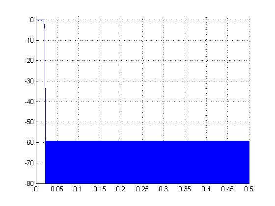
The order estimated by firpmord algorithm (n=1177) was incremented to 1178 to get a odd number of taps. I obtain -40dB at f=0.022 and -60dB at Fst aprox. (figure 3.20 upper-left).

[n,fo,ao,w] = firpmord([0.02, 0.02216],[1 0],[0.01 0.001],1);

h = firpm(1178,fo,ao,w); %very narrower transition band -> high order

Naming the integration of the magnitude spectrum (in linear scale) between Fst and (Fs/2) as 'int_bstop', and the integration between 0 and Fst as 'int_bpass', the relation in dB obtained was -36 dB.

Nfft = 2^16; %large number to get better approximation with trapz

HMAG = abs(fft(h,Nfft));

%integration of magnitude stopband

bin_stop =  1453; %the bin number for Fst

bins_stop = (bin_stop : Nfft/2);

freqs_stop = bins_stop*(Fs/Nfft);

mags_stop = HMAG(bins_stop+1);

int_bstop = trapz(freqs_stop,mags_stop);

%integration of magnitude passband

bin_pass = bin_stop-1;

bins_pass = 0:bin_pass;

freqs_pass = bins_pass*Fs/Nfft;

mags_pass = HMAG(bins_pass+1);

int_bpass = trapz( freqs_pass  ,mags_pass);

stop_pass_db = 20*log10(int_bstop/int_bpass) % integrate side-lobe ~-36 dB.

A new filter with a minimum stop-band attenuation -67.5dB give a integrate side-lobe level ~-45dB (I expected a value of -43.7dB).

astdb = 67.5; 

ast = 10^(-astdb/20);

[n,fo,ao,w] = firpmord([0.02, 0.02216],[1 0],[0.01 ast],1);

h = firpm(1320,fo,ao,w); 

The integrated sidelobes when the endpoints of the last filter are clipped was -53.7dB.

Hello jluqueq,

My compliments to you on the very sensible variable names in your MATLAB code. They made it easy for me to read your code. Based on my estimates of the filter's passband and stopband frequencies and your coding skills, it looks like your computed "integrated sidelobe level" is *VERY* similar to what fred harris predicted. Good job jluqueq!

(By the way, a bit of trivia. fred harris, a friend of mine, insists that his name be spelled with all lowercase letters. Check the spelling of his name on the front cover of his book.)

I hope you appreciated, as much as I did, harris' beautiful page 62 discussion of why we might want to clip the first and last coefficients of a high-order Parks/McClellan-designed FIR filter. harris is a true DSP guru. It's a shame that his book, filled with practical insights, is out of print.