


Understanding Subband Filtering?
Hi, I posted the following question on dsp.stackexchange.com recently but didn't get much of a response and was wondering if anyone here might be able to help.
In the past, I *believe* I've seen software that will decompose an audio signal (sampled at 44.1 KHz) into multiple different frequency bands. For example, I've seen where the signal is broken down, using an FFT, into the following subbands:
- Subband 0: Freq Range: 9,130.078 Hz to 22,050 Hz with 86.133 Hz per bin
- Subband 1: Freq Range: 4,651.17 Hz to 9,646.88 Hz with 43.066 Hz per bin
- Subband 2: Freq Range: 2,268.16 Hz to 4,909.57 Hz with 28.711 Hz per bin
- Subband 3: Freq Range: 1,062.30 Hz to 2,397.36 Hz with 14.355 Hz per bin
- Subband 4: Freq Range: 459.375 Hz to 1,126.904 Hz with 7.178 Hz per bin
- Subband 5: Freq Range: 190.210 Hz to 488.086 Hz with 3.589 Hz per bin
- Subband 6: Freq Range: 52.0386 Hz to 206.360 Hz with 1.794 Hz per bin
- Subband 7: Freq Range: 0.8972 Hz to 60.114 Hz with 0.8972 Hz per bin
I understand where the first subband (subband 0) comes from - it's simply a 512 point FFT applied to a 512 sample window of the digital audio. This results in 256 frequency bins, each with 86.133 Hz per bin. However, I'm not understanding how the remainder of the bands are created.
To create subband 1, I could of course take a 1024 point FFT of 1024 sample window instead of 512, and then for subband 2 I could take a 2048 sample window of 2048 samples, and then so and and so forth for the other bands.
However I'm pretty sure there is some way to generate all of the subbands using only the same 512 samples that were used to create subband 0. I'm just not sure how.
To phrase it another way: Is there anyway for me to get the continually finer resolution (i.e. smaller size frequency bins) I get in subbands 1-7 from just the original 512 digital audio samples?
When I posted this on dsp.stackexchange.com the only feedback I got was that there is no way to get finer resolution if you keep the FFT length (points/samples) and sampling rate unchanged. And that I should look at en.wikipedia.org/wiki/Filter_bank#Multirate_Filter_Bank
I read through and studied the Wikipedia link. I understand I'm supposed to change the sample frequency of the input to a lower sample rate and therefore will get better frequency resolution when doing the FFT, but since the signal is already in discrete/digital form, lowering the sample rate will not accomplish anything.
For example, I could downsample the original 512 sample input window in half from 44.1 KHz to 22.05 KHz, but this will reduce the window sample size from 512 samples to 256 samples and therefore result in frequency bins with the same resolution as before (86.133 Hz per bin).
I must be misunderstanding something here. I would be very appreciative if anyone could explain this. Thank you.

Hello,
Although I don't work with multirate filters on a daily basis, I think I can provide you with some insight on what is going on here.
In order to apply a 512-point FFT across all of the subbands you need to apply two ordered operations to a signal: 1.) bandpass filtering and 2.) down-sampling of the filtered signal. By using these two operations, you can decrease the effective sample rate of the signal found in each subband. A smaller sample rate, in conjunction with a constant FFT size of 512-points, will improve the resolution of the FFT bin-size.
Consider the following Matlab code,
%% Environment

close all; clear; clc;
set(0, 'DefaultFigureWindowStyle', 'normal');


%% Decimation Factors

fs=44.1e3;
decimationFactors=[  1, 2, 3, 6, 12, 24, 48, 96  ].';
fftSize=512;
[fs./decimationFactors./fftSize decimationFactors]


%% Test Signal

netTime=1.0; timeIndices=0:1/fs:netTime-1/fs;
s=sin(2*pi*10*timeIndices)+0.5*cos(2*pi*20*timeIndices)+0.65*sin(2*pi*40*timeIndices)+sin(2*pi*10e3*timeIndices);
%
[ MX, f ] = fourier( s, fs, fftSize );
figure; plot(f, 20*log10(abs(MX))); title(sprintf('Original Signal\n(Bin size: %5.4f Hz)', fs/fftSize)); xlabel('Freq. (Hz)'); ylabel('Amp. (dB)'); axis([-5e2 fs/2 -100 5]); grid on; shg;


%% Filtering with Subband Filter 7 and Decimation

% https://www.mathworks.com/help/signal/ref/butter.h...

[z, p, k] = butter(4, [0.8972 60.114]./(fs/2), 'bandpass'); sos = zp2sos(z, p, k);
% figure; freqz(sos, 4096, fs);

sFiltered=sosfilt(sos, s);
[ MX, f ] = fourier( sFiltered, fs, fftSize );
figure; plot(f, 20*log10(abs(MX))); title(sprintf('Bandpassed Filtered Signal Prior to Decimation\n(Bin size: %5.4f Hz)', fs/fftSize)); xlabel('Freq. (Hz)'); ylabel('Amp. (dB)'); axis([-5e2 fs/2 -100 5]); grid on; shg;

sFilteredDecimated=downsample(sFiltered, 96); decimatedFs=fs/96;
[ MX, f ] = fourier( sFilteredDecimated, decimatedFs, fftSize );
figure; plot(f, 20*log10(abs(MX))); title(sprintf('Bandpassed Filtered Signal After Decimation by 96\n(Bin size: %5.4f Hz)', decimatedFs/fftSize)); xlabel('Freq. (Hz)'); ylabel('Amp. (dB)'); grid on;


%% Decimation Without Filtering

sFilteredDecimated=downsample(s, 96); decimatedFs=fs/96;  % Note:  If you use the "decimate.m" function, it will apply a lowpass Chebyshev Type I IIR filter of order 8.
[ MX, f ] = fourier( sFilteredDecimated, decimatedFs, fftSize );
figure; plot(f, 20*log10(abs(MX))); title(sprintf('Decimated Signal w/o Bandpass Filtering\n(Bin size: %5.4f Hz)', decimatedFs/fftSize)); xlabel('Freq. (Hz)'); ylabel('Amp. (dB)'); grid on;


%% Arrange Figures

autoArrangeFigures(2, 4, 2);


%% References

% https://en.wikipedia.org/wiki/Filter_bank#Multirat...
In this example I have created a signal composed of tones at 10 Hz, 20 Hz, 40 Hz, and 10 kHz at a sample rate of 44.1 kHz.
If I take a 512-point FFT at 44.1 kHz, the tone at 10 kHz is readily visible (bin size is approximately 86.1328 Hz) as shown in this figure.
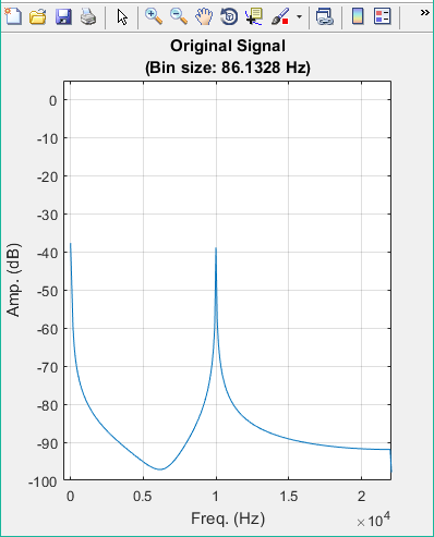
However, the tones at 10, 20, and 40 Hz are clearly not visible.
To rectify this problem, we can design and apply a bandpass filter for subband 7 and decimate the bandpass filtered signal. I designed a 4th-order Butterworth filter (maximally flat in the passband) using the 0.8972 Hz and 60.114 Hz frequencies as the 3-dB cut-off frequencies and filtered the original signal. This process removes the 10 kHz tone as shown in the following figure.

Note that the spectral resolution of the FFT has not changed (approximately 86.1328 Hz) and again does not allow the 10, 20, and 40 Hz tones to be seen. But since we have removed the 10 kHz tone, the signal can now be down-sampled (i.e. decrease the effective sample rate) to improve the resolution of 512-point FFT. This is what kaz indicated in his response.
To achieve the FFT resolutions with a 44.1 kHz sample rate in your post, decimation factors of [ 1, 2, 3, 6, 12, 24, 48, 96 ] are needed. Since we are looking at subband 7, a decimation factor of 96 is used to down-sample the bandpass filtered signal.
The 512-point FFT of the original composite tone signal after bandpass filtering and down-sampling by a factor of 96 is shown in Figure 3 below.

As you can see, the 10, 20, and 40 Hz tones are now visible.
If you had down-sampled the original signal without first filtering it, the 10 kHz tone would have been alaised as shown in Figure 4 below.

The effective sample rate after decimation by a factor of 96 is approximately 459.3 Hz. If the 10 kHz tone is not removed by filtering prior to down-sampling of the original signal, it will be aliased to a frequency of about 105.9 Hz, which is shown in the previous figure.
If you are working with Matlab, an important item to remember is that there are multiple ways of down-sampling, or decimating (i.e. the removal of samples), a signal. In my Matlab code, I used the function "downsample". This function just drops samples without any other processing. However, there is another function called "decimate" that will apply a filtering operation to the signal prior to dropping samples from the signal. This is done to prevent aliasing.
As I indicated, I don't work with multirate filtering on a regular basis, but I think I have captured the essential ideas of the method. I know there are more elegant ways of realizing this process, but I cannot provide specific examples or references right now.
I hope this helps,
Michael.
Hi Michael - Thanks so much for the detailed explanation. I haven't used MatLab before (I usually use C/C++) but looking through the code you've posted and your explanations, I think I understand.
Please correct me if I'm wrong, but it appears your general process is:
1) Lowpass the signal (to prevent aliasing when downsampling)
2) Downsample the signal
3) Perform FFT and now you have better resolution due to the lower sample rate
I understand this process, and have used it before. However, in this case, I'm wanting to keep the time window fixed so I know what frequencies exist in that exact 11.6 milliseconds (44100 / 512).
Looking at your example, I'm pretty sure you're now looking at a much longer duration of the input signal - basically 1.11 seconds (459.3 / 512).
Or am I missing something?
Using Micheals (awesome, btw) example, 11.6ms is not enough data to discriminate the lower frequencies. This should make intuitive sense because the period of 10 Hz is 100ms. You could use a bigger window, but the FFT may become too computationally expensive to be practical. By breaking the signal into Subbands with different sample rates, you can get the frequency resolution you need in each band independently of each other
Hello,
The effective duration of the signal before and after decimation is unchanged. The original signal, "s", is 1 second in duration (i.e. see the "netTime" variable). The decimated signal is slight longer, but has approximately the same duration (i.e. 460 samples /(44.e13 / 96) or 1.0014 seconds; the denominator (44.1e3/96) is the new sample rate of the decimated signal).
Because the sample rate changes and the size of the FFT does not change (i.e. a 512-point FFT), the bin size of the FFT changes from 86.1328 Hz to 0.8972 Hz. Again, this allows the 10 Hz, 20 Hz, and 40 Hz tones to be resolved and visible in the spectra.
I believe you are confusing the change in sample rate with the corresponding change in FFT bin size and the unchanged duration of the signal pre- and post-decimation.
To recapitulate, the length of the pre-decimated signal is 44.1e3 samples (i.e. 1 second at 44.1e3 samples per second). The length of the post-decimation signal is 460 samples. The durations of the pre- and post-decimated signals are, respectively, 44.1e3 samples / 44.1e3 samples per second or 1 second and 460 samples / (44.1e3 samples per second / 96 ) or approximately 1.0014 seconds for the post-decimated signal.
Another idea that comes into play here is the Zoom-FFT. See Signal Processing forum and Comp.dsp forum threads that discuss this topic. The second link might provide you with C/C++ code to compute Zoom-FFT (i.e. "Basic Principal of the Zoom FFT".
Michael.
Thank you again, Michael. It is clear to me that I'm not entirely grasping what you say, but spending some time thinking about what you've said here and referencing the sources you've mentioned I believe stand a good chance of helping me understand.
I have a very busy week at work (DSP is my hobby), but will get to this later in the week and reply back with what I've found.
Thank you again for the your very generous assistance.
Hello,
No problem. My pleasure. Please keep in touch.
Michael - Thanks for the above information. Apologies for the delayed response. As mentioned in another place on this thread, I started a new job last Monday (I'm a software engineer) and that has kept me busier than usual all through the past week.
This weekend I read through your last post and the links in detail and I think the Zoom FFT just might be the solution I'm looking for.
This link: https://www.arc.id.au/ZoomFFT.html appears to be most helpful. I'm not yet grasping the process 100%. I need to refresh myself on amplitude modulation.
I've never really used amplitude modulation for anything in my DSP adventures, but I do recall studying it when reading through "The Scientist and Engineer's Guide to Digital Signal Processing" a few years back.
I'm going to review this chapter and go from there.
Thanks again, I really appreciate the help and information you've provided.
If anyone is interested in my progress with this over the next few weeks please feel free to post to this thread and ask. I will be happy to provide updates.
-Terence
One more item, if you do not have access to Matlab, Octave is an great alternative. See "https://www.gnu.org/software/octave/".

Hi,
Without going into details of your case I would like to comment on your assumption that
"but since the signal is already in discrete/digital form, lowering the sample rate will not accomplish anything".
You can lower it for the sake of 512 fft resolution since fft bin resolution is sampling rate/number of bins
Hi Kaz - Thanks for the reply. I must be misunderstanding something. Let me explain how I understand it:
I have 512 samples that have been sampled at 44100 Hz. I can (using resampling) convert the 512 samples into 256 samples at 22050 Hz sample rate, however, since I then only have 256 samples, I must perform a 256 FFT and cannot do a 512 FFT. Because of this, I still end up with sample bin sizes in the frequency domain exactly the same size as before: 86.133 Hz per bin.
Am I missing something?
You downsample to half rate but still should have enough of signal to go for 512 samples. Otherwise your case is too restrictive and you may try insert zeros but I am not going that way inserting 256 zeros
Thanks, Kaz. Yeah, I'm wanting to keep the time window fixed to so I know what frequencies exist in that exact 11.6 milliseconds (44100 / 512). And yes, referencing one of my DSP books, I did try zero stuffing but did not get the results I hoped for.
One other way is to repeat the downsampled section twice. This should give the same frequencies as one section with a bit of windowing tricks at the edges if too sharp
That is not a bad idea. Let me give that a try and I'll report back.
Apologies for the delayed response. I started a new job last Monday (I'm a software engineer) and that has kept me busier than usual.
So, I tried this approach.
I first created an input signal containing two low frequency notes: C2 (65.41 Hz) and E2 (82.41) at a sample rate of 44100 Hz.
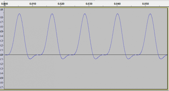
Here's an example of the beginning of what the signal looks like:
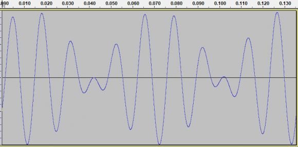
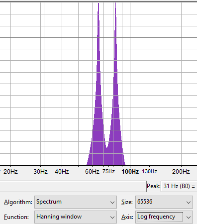
Taking just the first 512 samples, applying a Blackman window and repeating the samples ends up with (unsurprisingly) a very different waveform in the time domain:
...and just as unsurprisingly, very different frequency domain results:
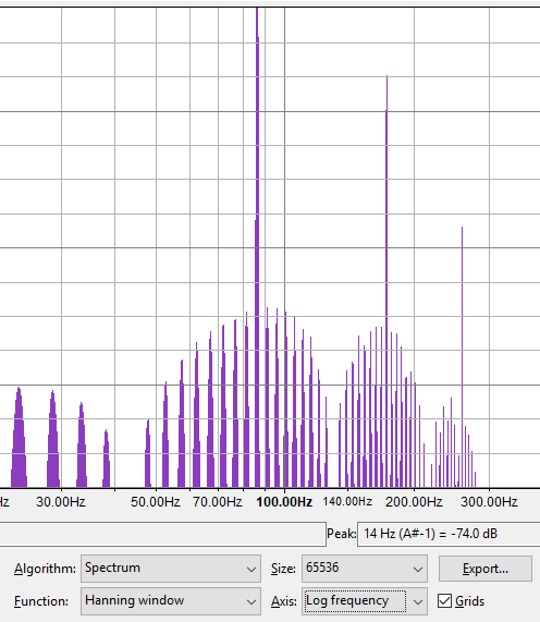
:(
your f1 and f2 are too low and their separation is too low for 512 fft resolution.
a resolution of 512 means bin resolution of 44100/512 = 86 Hz yet your f1-f2 = 82-65 = 17 Hz
Yes, I see... And this leads me back to my original thought that this is just not possible with such a limited number of samples.
My goal is to be able to have high resolution in the frequency domain to tell what different notes appear in the audio signal, but also have a short time duration since notes could change as rapidly as once every 25 milliseconds.
To phrase it a different way: I want to know what notes (i.e. frequencies) are present in every 25 milliseconds of an audio signal.
Example of what frequencies notes are in the lower end of the spectrum:
| Note | Frequency (Hz) |
| C1 | 32.70 |
| C#1/Db1 | 34.65 |
| D1 | 36.71 |
| D#1/Eb1 | 38.89 |
| E1 | 41.20 |
| F1 | 43.65 |
| F#1/Gb1 | 46.25 |
| G1 | 49.00 |
| G#1/Ab1 | 51.91 |
| A1 | 55.00 |
| A#1/Bb1 | 58.27 |
| B1 | 61.74 |
| C2 | 65.41 |
| C#2/Db2 | 69.30 |
| D2 | 73.42 |
| D#2/Eb2 | 77.78 |
| E2 | 82.41 |
| F2 | 87.31 |
| F#2/Gb2 | 92.50 |
| G2 | 98.00 |
| G#2/Ab2 | 103.83 |
| A2 | 110.00 |
| A#2/Bb2 | 116.54 |
| B2 | 123.47 |
| C3 | 130.81 |
If you have to use 512 resolution then lower Fs well below 44100Hz so that you get the required resolution. That is decimate using appropriate filtering and then use 512 samples (or repeat if you end up with fewer samples).


