


Large image - https://postimg.org/image/c74zc1b9z/
Download image https://s31.postimg.org/4eebk25ax/cookbook_comp.png?dl=1
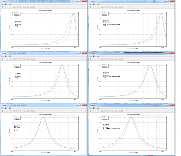
Right column plots uses EE's Q definition just for the (original) cookbook. Did not check the situation of phases yet.
If my plots are correct then it looks like prewarping Q might bring some improvement at least for peak filter magnitude. For LP filter, situation is different.
BTW, some doctoral thesis showed plots where both prewarpings were used and set to have equal factor. How's that factoring done?
Any thoughts?

alright, there are a couple of different issues that may (or may not) need to be de-conflated.
i'm gonna try to keep the number of symbols minimized.
\(dB_\text{gain}\) is the number of dB gain of the peak (for \(dB_\text{gain} > 0\)) or cut (for \(dB_\text{gain} < 0\)). appears to be 6 dB in the plots.
$$A^2 \triangleq 10^{dB_\text{gain}/20}$$
is the linear gain for the boost or cut.
\(f_\text{s}\) is sample rate.
\(f_0\) is frequency of the boost or cut in the same units as the sample rate.
the analog transfer function of a resonant second-order filter (a.k.a. "biquad" or "SOS") is
$$\begin{align} \\ H(s) &= \frac{b_0 + b_1 s + b_2 s^2 }{1 + a_1 s + a_2 s^2} \\ \\ &= \frac{b_0 + b_1 s + b_2 s^2}{1 + \frac{1}{Q}\frac{s}{2 \pi f_0} + \left(\frac{s}{2 \pi f_0} \right)^2} \\ \\ \end{align} $$
don't conflate the \(a_k, \ b_k\) coefficients of the analog prototype with those in the resulting digital filter from the recipe in the cookbook. this is how the "EE definition" of \(Q\) is defined.
an analog BPF with passband gain of 0 dB, has transfer function:
$$ H(s) = \frac{ \frac{1}{Q}\frac{s}{2 \pi f_0} }{1 + \frac{1}{Q}\frac{s}{2 \pi f_0} + \left(\frac{s}{2 \pi f_0} \right)^2} $$
note when \(f = f_0\) then \(H(j 2 \pi f_0) = 1\). note also that there are two bandedges \(f_+\) and \(f_-\) such that \(f_- < f_0 < f_+\) and
$$ f_+ = f_0 \cdot 2^{bw/2} $$ $$ f_- = f_0 \cdot 2^{-bw/2} $$
and
$$ |H(j 2 \pi f_-)|^2 = |H(j 2 \pi f_+)|^2 = \frac{1}{2} $$
we define those bandedges for the BPF to be the "half-power frequencies". and the \(BW\)parameter is the bandwidth expressed in octaves. the higher bandedge \(f_+ = 2^{bw} f_-\) is \(BW\)octaves higher than the lower bandedge \(f_-\). turns out that this bandwidth is related to Q as follows:
$$\begin{align} \\ \frac{1}{Q} &= \frac{2^{bw} - 1}{2^{bw/2}} \\ \\ &= 2 \ \sinh \left( \frac{\ln(2)}{2} \ bw \right) \\ \end{align} $$
keeping the same definition of \(Q\), the "bell-shaped" boost/cut parametric EQ takes that BPF, gives it some gain (with sign) and adds it to a wire. it has transfer function:
$$\begin{align} H(s) &= (A^2 - 1)\frac{ \frac{1}{Q}\frac{s}{2 \pi f_0} }{1 + \frac{1}{Q}\frac{s}{2 \pi f_0} + \left(\frac{s}{2 \pi f_0} \right)^2} \ + 1 \\ \\ &= \frac{1 + \frac{A^2}{Q}\frac{s}{2 \pi f_0} + \left(\frac{s}{2 \pi f_0} \right)^2}{1 + \frac{1}{Q}\frac{s}{2 \pi f_0} + \left(\frac{s}{2 \pi f_0} \right)^2}\\ \end{align}$$
that is the "traditional" analog parametric EQ. note that $$|H(j 2 \pi f_0)| = A^2 = 10^{dB_\text{gain}/20}$$ problem is that, leaving \(f_0\) and \(Q\) constant, the curve for \(dB_\text{gain} > 0\) is not a mirror image for \(dB_\text{gain} < 0\), given the same magnitude \(|dB_\text{gain}|\). the cut will be much skinnier than the boost.
some people might want the cut to exactly undo the boost given all other parameters being the same. so in the cookbook (and in some other papers), a redefinition of \(Q\) is made. this redefinition is the substitution:
$$ Q \ \leftarrow \ A \cdot Q $$
so that makes the transfer function for the parametric EQ (with adjusted \(Q\)):
$$\begin{align} H(s) &= \frac{1 + \frac{A^2}{A \cdot Q}\frac{s}{2 \pi f_0} + \left(\frac{s}{2 \pi f_0} \right)^2}{1 + \frac{1}{A \cdot Q}\frac{s}{2 \pi f_0} + \left(\frac{s}{2 \pi f_0} \right)^2} \\ \\ &= \frac{1 + \frac{A}{Q}\frac{s}{2 \pi f_0} + \left(\frac{s}{2 \pi f_0} \right)^2}{1 + \frac{1}{A \ Q}\frac{s}{2 \pi f_0} + \left(\frac{s}{2 \pi f_0} \right)^2} \\ \end{align} $$
note that if \(dB_\text{gain}\) is replaced with \(-dB_\text{gain}\), then \(A\) is replaced with \(\frac{1}{A}\) and the numerator and denominator are essentially swapped, which causes the frequency response of the cut to mirror that of the boost.
now, using the same relationship between bandwidth \(BW\)and \(Q\):
$$ \frac{1}{Q} = 2 \ \sinh \left( \frac{\ln(2)}{2} \ bw \right) $$
then the bandedges
$$ f_+ = f_0 \cdot 2^{bw/2} $$ $$ f_- = f_0 \cdot 2^{-bw/2} $$
satisfy this gain definition:
$$ |H(j 2 \pi f_-)| = |H(j 2 \pi f_+)| = A = 10^{dB_\text{gain}/40} $$
which is the "mid-gain frequency" having gain of \(\frac{dB_\text{gain}}{2}\).
so the definition of bandedge gain is a bit different, but at least for the analog prototype, we're keeping the relationship between \(BW\)and \(Q\) the same. higher \(Q\) means tighter \(bw\).
so, first, before we discuss "warping Q", let's be completely consistent about which Q to compare. for this, i might recommend leaving the "EE definition" of Q behind to not confuse.
so the bilinear transform that compensates for the frequency warping at the "significant frequency" or the resonant frequency \(f_0\) makes this substitution:
$$ \text{normalized }s \triangleq \frac{s}{2 \pi f_0} \ \leftarrow \ \frac{1}{\tan(\pi f_0/f_\text{s})} \ \frac{1 - z^{-1}}{1 + z^{-1}} $$
\(H(z)\) is the resulting digital filter transfer function after making that substitution for normalized \(s\).
and that does not compensate for a cramped bandwidth because, besides the resonant frequency \(f_0\), so also are the bandedges \(f_+\) and \(f_-\) warped by the bilinear transform. measured in octaves the bandwidth, \(BW\), in the digital filter is:
$$\begin{align} BW &= \log_2\left( \arctan\left(\frac{\pi f_+}{f_\text{s}}\right) \right) - \log_2\left( \arctan\left(\frac{\pi f_-}{f_\text{s}}\right) \right) \\ \\ &= \log_2\left( \arctan\left(\frac{\pi f_0 2^{bw/2}}{f_\text{s}}\right) \right) - \log_2\left( \arctan\left(\frac{\pi f_0 2^{-bw/2}}{f_\text{s}}\right) \right) \\ \end{align}$$
you can see that the mapping of \(bw\) to \(BW\) is an odd-symmetry function, so it goes through \(0\) and has no even-order terms in a Maclaurin (a.k.a. Taylor series) expansion. now if you fix \(f_0\) and plot digital \(BW\)vs. analog \(bw\), you will see that \(BW < bw\) and that is the bandwidth cramping done by frequency warping of the bilinear transform. to uncramp the bandwidth, you would have to solve for \(BW\)in terms of \(BW\)and \(f_0\) and \(f_\text{s}\). and that is (how shall we say?) a female canine.
if you read the cookbook a little, you will notice a slightly adjusted mapping between \(BW\)and \(Q\):
$$ \frac{1}{Q} = 2 \ \sinh \left( \frac{\ln(2)}{2} \ BW \frac{2 \pi f_0/f_\text{s}}{\sin(2 \pi f_0/f_\text{s})} \right) $$
so the digital filter bandwidth \(BW\)was increased by a factor of \(\frac{2 \pi f_0/f_\text{s}}{\sin(2 \pi f_0/f_\text{s})}\) as a first-order attempt to compensate for the bandwidth cramping. this result comes from assuming a narrow bandwidth in the first place and evaluating the derivative:
$$ \frac{d \ BW}{d \ bw} \Bigg|_{bw = 0} = \frac{\sin(2 \pi f_0/f_\text{s})}{2 \pi f_0/f_\text{s}} $$
the first term of the Maclaurin series is
$$ BW \approx \frac{\sin(2 \pi f_0/f_\text{s})}{2 \pi f_0/f_\text{s}} bw $$
compensating (or "prewarping") that first-order cramping of the bandwidth (which is what i think you mean by "prewarping Q") is done in the cookbook and always has been. but it is only a first-order compensation. if you want to do it better, be my guest and try to compute the next third-order term for the Maclaurin expansion (and flip it around so you have an expression of the approximate analog \(BW\)in terms of digital \(bw\)). doing this with Maclaurin series expansion is the only way i know because i don't think you will invert the \(bw \to BW\) mapping above directly.
Thanks for answering here too.
I did plot the peak filter build through cookbook's "case BW" instead of "case Q". It gave better magnitude response.
'Prewarping' Q improved the magnitude response when filter was build through "case Q".
Plots showing the end results for this thread.

Large image direct link https://postimg.org/image/akaptb335/

It looks like it might be interesting, but:
- Graphs are too small too read
- TLA density is way too high -- what does "turning into II" mean? What do bacon, lettuce and tomato sandwiches have to do with digital signal processing? Who's "EE"?
It may all be totally clear if the graphs were large enough that you could read their text -- but you should still unpack the three-letter abbreviations.
Is there a way prevent this forum software from shrinking the image (original is W=1752px X H=1513px)? I'll add link to some picture sharing site.
Abbreviation 'EE' comes from RBJ's Audio EQ Cookbook (linked in post #1).
II means Impulse Invariant.
I don't know about picture shrinking, but if you had the patience you could post six photos.
(Other sites that I'm on post a thumbnail with a link to the bigger picture -- but that'd be considerable work.)

Is there a way prevent this forum software from shrinking the image?
Unfortunately no, for the moment. I'll add the option to upload large images on my list of improvements to be implemented. Thanks.


