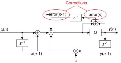
I'm reading the 3rd edition of Richard Lyons' excellent book and am a bit confused by the DC-removal filter in Figure 13-65(b). If the input to the quantizer Q is an "accumulator" value q(n) and its value is higher than what can be represented in the width of y(n), then error(n) is positive; so wouldn't we want to subtract that error from the accumulator in the next cycle? As it is shown, the quantization error is *added*, which means y(n) will saturate even more.

I have a C++ model and if I reverse the sign of error(n-1) coming into that adder, it gracefully handles the over-range q(n) signal to produce only a single saturated y(n) sample, but if I implement the filter as drawn, the output y(n) clips. Or, maybe I'm misunderstanding somthing.

For reference, his figures are also posted here:

https://www.embedded.com/design/configurable-syste...

Here is an example adding large offsets to a sine wave, using 2.30 fixed point. The yellow curve shows the clipped output before, and not clipped after making the change in quantization-error-sign. I wasn't sure how to put an image in this forum post, so the comparison is hosted here:

https://imgur.com/a/gDWBrhP

Hi swirhun.

I'm not ignoring you. I will go through my modeling software code for Figure 13-65(b) and see if I've made some sort of coding error. I'll get back to you.

While I'm reviewing my code, will you tell me what are the definitions of the colored curves in your two 'imgur.com' images? (The legend in your top image is unreadable.)

[-Rick Lyons-]

 

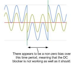
Thanks Rick; no rush at all. Sorry those images didn't work so well; I now have fuller access to the forums so I am trying to attach a better image now. Blue is the input, Red is the quantization error, Yellow is the output, and Dotted Green is the accumulator before quantization. The accumulator value is pretty much the same as the output, except where the overflow occurs at those steps. Let's see if these images come through: they are the results after you reverse the sign of error(n-1) in the figures:

Screenshot 2018-08-17 at 11.21.46 PM.png

Screenshot 2018-08-17 at 11.22.21 PM.png

Also, don't take the plots too seriously; they're quick spreadsheet-based plots using Google Sheets. The input and output are 2.30 fixed point (I'm using algorithmic C types ac_fixed for HLS), so the range is [-2.0, +2.0-quantum]. I know the plot shows the yellow curve going a bit above +2.0 but that's just a graphical artifact.

And here is the result as drawn in the figure. You can see I've chosen saturating arithmetic for the output so it clips (rather than wrapping around). Still, I think the point of this filter is to avoid the need for wider output word than you have input word.

Screenshot 2018-08-17 at 11.34.15 PM.png

Have a good weekend,

-Paul

Apologies If I going off track but an alternative that we use in FPGAs to avoid dc of truncation is to round up using "unbiased rounding" rather than pass the error to next sample. 

The unbiased rounding is normal rounding but the midpoints fractions(.5) are treated differently depending on lsb of sample value being even or odd. That way the error of midpoint fractions is spread at random.

Hello Paul.

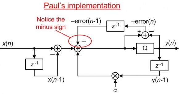
I've been checking my MATLAB code that modeled the filter in my Figure 13-65(b), and I could find to errors in that code, so far. However, thanks to you I see a necessary correction in Figure 13-65(b). My original signal labels ('error(n-1)' & 'error(n)') are missing minus signs. The corrected figure is the following:

My mistake was calling signal '-error(n-1)' a positive error when in fact it is a negative error. So the upper feedback path is NOT adding a +error to the center adder (the accumulator). The upper feedback path is adding a negative error ('-error(n-1)') to the center adder. Thus I'm actually subtracting a positive error from the center adder.

If I understand you correctly you are implementing the following filter:

When I model your implementation using 16-bit words I notice that your implementation does reduce the unwanted DC bias of the input signal but some DC bias still remains in your output. When I model your implementation using 8-bit words a significant amount of DC bias remains in your implementation's output.

Looking carefully at your 'Screenshot 2018-08-17 at 11.21.46 PM.png' image I detect a small amount of remaining (unwanted) DC bias in your filter's output signal as shown below:

Paul, instead of using 32-bit words in your implementation, are you able to use 8- or 10-bit words to verify my suspicion that your implementation does not fully remove an input signal's unwanted DC bias?

I'm not sure I follow that reasoning. If you look at the filter as drawn in the textbook ("Screenshot 2018-08-17 at 11.34.15 PM.png") there is a gigantic DC offset that makes its way through the filter when an offset is added to the input. My version with the minus sign added as you have drawn, has only a tiny offset.

If you use more integer bits in the output, then instead of clipping, the output follows the accumulator. However, this happens even if you didn't include any quantizer. The textbook indicates that this architecture with the quantizer allows you to avoid the word-width growth.

To be more specific, I don't understand your point. There is a much larger DC offset in the original implementation. I've annotated it with an arrow similar to how you have done for my version:

qKJY8bowe4z.png

I decided to derive the transfer functions to see if that helps me understand it at all. Sorry if the forum spams you a few times while I edit these Latex equations. Quantization means A-Y=E, so the error(n) signal ("E") is positive because Y < A when you lop off LSBs. "A" is the accumulator, which is what I'm calling the input of the quantizer in Fig 13-65(b). The error E is subtracted in the quantizer operation, and a delayed version of E is added to the accumulator A in the textbook's figure. The only difference in my example is the sign with which the delayed version is added to the accumulator: basically I wondered if we should subtract it instead of add it.

Assuming superposition of the quantization error and signal (for simplicity)

For both versions, the signal transfer function is the same:

<$$ \frac{Y}{X} = \frac{1-z^{-1}}{1-\alpha z^{-1}} $$>

For the original figure's (+) sign:

$$ \frac{Y}{E} = \frac{-1+z^{-1}}{1-\alpha z^{-1}} $$

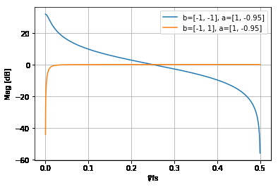
If you reverse the sign to (-) the only thing that changes is the delayed error term in the numerator:

$$ \frac{Y}{E} = \frac{-1-z^{-1}}{1-\alpha z^{-1}} $$

The freqz style magnitude plots of those error transfer functions are below. I'm not totally sure how to interpret these because the quantization error is not a periodic signal. But, it looks like the textbook's version (orange curve) knocks out the DC error and otherwises passes it to the output. Changing the sign appears to amplify it below Fs/4, and attenuate it above Fs/4. While this looks bad at low frequencies, the quantization error doesn't actually "hang out" at low frequencies; if it is really uncorrelated to the signal, it probably has a white frequency spectrum.

Here are a few thoughts / discussion ideas:

- This ignores the "overflow" issue where the added minus sign appears to do better: empirically, it prevents clipping. I don't think this is represented in the transfer function plot though.

- Perhaps the answer is whichever integrates to lower total output power? That would assume the quantization error is white.

- Maybe you can implement a hybrid version of both signs using a little logic. Basically, implement the figure as drawn in normal operation, but if the accumulator exceeds the capacity of the output, you flip the error sign for one cycle to avoid clipping. This would basically "reset" the removal of the output's DC component to prevent clipping.

- I guess the null at zero frequency in the original figure shows that it "dithers" rather than sitting at some static quantization error. This is the noise modulating effect we expect to see from recycling the error, like in a delta-sigma modulator.

Feel free to correct me if I'm misinterpreting something...

Hello Paul (I'm replying to your 8/20/2018 post that begins with the words: "To be more specific,...").

When I look at your nice image (qKJY8bowe4z.png) produced by your implementation of my Figure 13-65(b), it appears to me that the DC removal filter is working properly. Referring to the following annotated version of your image: during Period# 1 the Figure 13-65(b) filter output (green curve) is indeed approaching a DC offset of zero, as it should.

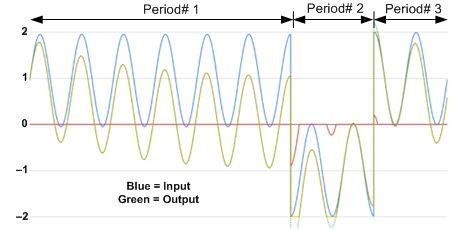
During Period# 2 the filter output (green curve) is trending toward a DC offset of zero. During Period# 3 the filter output (green curve) is again trending toward a DC offset of zero. So all of this leads me to think the Figure 13-65(b) filter is working properly.

Paul, in your code that produced your image qKJY8bowe4z.png, can you extend (lengthen) the time durations of Periods# 1, 2, and 3 to see if the Figure 13-65(b) filter's output does indeed trend toward and eventually achieve a DC offset of zero amplitude?

[-Rick-]

Ah, that makes sense, so you're just referring to the exponential trend towards zero. Yes, I can lengthen those times and check it out, but I think my spreadsheet-based plotter is probably not up to the challenge.

I extended all time periods by 100x. They both have the same qualtative behavior of trending towards zero. The average signal values in the "stepped down" region (over 100k samples) are:

error=-4.64923296e-10

accum=-1.93874816e-06

input=-9.90000000e-01

output=-1.93921309e-06

Using the original (+) sign for the error, the plots look similar, but the output actually does average to zero, as you indicated earlier...

error = 4.77769626e-10

accum = 4.77769349e-10

input = -9.90000000e-01

output = 0.00000000e+00])

I think this is explained by the transfer functions I derived earlier for the quantization error. The original transfer function has a gain of Y/E = 0, and my sign-modified version has a DC gain of Y/E = 2/(1-alpha) = 72.40742956889684 dB (my simulation uses alpha=0.99952064361423254000).

Due to two's complement arithmetic being asymmetrical, the average value of 2.30 fixed-point math is not 0 but is actually -0.5/(2**30) = 4.656612873077393e-10, so combined with the Y/E gain at DC, that would produce an output DC offset of 1.9428604734750975e-06, which is pretty darn close to what I observed above.

Anyway, thanks for the guidance on this. I guess the figure is correct as-is, and we just have to deal with the clipping (or wider output word) for pathological inputs like this full-range input step.

Although the sign flip I proposed fixes the overflow issue by immediately "resetting" the acccumulator's DC value whenever a signal would clip, it probably also screws up the quantization-noise-modulating properties and introduces a small DC error due to nonzero quantization-error gain (Y/E) at DC.

Hi Paul.

Referring to your 8/20/2018 post that starts with: "I decided to derive...", your idea of finding the "Y(z) divided by E(z)" error transfer function is a good idea. Using the filter shown in Part (a) of the below figure (my book's Figure 13-65(b), I was also able to derive your Y(z)/E(z) transfer given in Part (b) of the below figure.

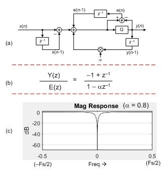
Part (c) of the above figure gives the frequency magnitude response of the Y(z)/E(z) transfer function (when alpha = 0.8). That freq magnitude response has the desired deep notch at zero Hz (Y(z)/E(z) has a z-domain zero at z = 1). That way, the quantizer contributes no DC component to the y(n) output of the Part (a) DC removal filter.

Referring to your 8/20/2018 post that starts with: "Anyway, thanks for the guidance...", it appears that you and I agree that my book's Figure 13-65(b) is correct.

Paul, this thread forced me to "dig deeper" in understanding the behavior of my Figure 13-65(b) filter. That's to my benefit so I'll say "Thanks" to you for your original post on 8/17/2018.

[-Rick-]

Hi Rick, Paul,

With due respect for your useful posts I am a bit unsure about some issues discussed here.

Firstly: The issue of truncation dc bias is better avoided by proper rounding - in my opinion - than allowed to be mitigated. This is a well accepted paradigm in design methodology. Your method will simply add dither to the signal.

Secondly: The issue of truncation is mixed up with overflow in a way that doesn't look right to me.

Thirdly: The theme is about truncation bias yet the examples given show dc offset over a segment of signal. 

Kaz

Hi Kaz,

I'm definitely open to your suggestions. All you said was "round it" though. Even with rounding, you get truncation error, but it's just half the magnitude and signed. Do you have any specific corrections to add to the points made above? You think I should avoid the truncation noise feedback and just round to the final resolution?

Thanks,

Paul

Rounding can be of several types:

1) direct truncation: just discard LSBs. This leads to dc bias (floor in matlab) and can build up in accumulators.

2) rounding to nearest integer: This is ok with dc if there is no overall dc offset i.e. there is equal negative and positive probability.(round in Matlab)

If there is dc offset then a tiny extra dc builds due to midpoint fractions being rounded in one direction.

The midpoint bias increases as less bits are to be discarded reaching 50% if only 1 lsb is to be discarded.

3) best is rounding to nearest even(or nearest odd) (convergent in matlab). No dc occurs here as midpoints are spread with even/odd having same probability. Also known as dc unbiased rounding.

Example vhdl algorithm for 3, discarding 15 bits off 31 bits to get 16 bits:

truncated_result <= result(30 downto 15);

if result(14) = '1' then  -- fraction of 0.5 or more

   if result(15 downto 0) /= "0100000000000000" then --not even&exact .5

         truncated_result <= result(30 downto 15) + 1;

   end if;

end if;

I haven't seen VHDL used (in the USA), but I mostly get it. So when truncating N bits off, you round up if X[N-1] is 1 and X[N:0]/(2**(N-1)) is greater than or equal to 1? [Note: I made several edits to this forum post as I refined that formula]. I don't immediately see how that solves the quantization error issue, but I probably just have to go through a numeric example.

I'm actually not using Verilog either. I'm using HLS, which has rounding types explained in Table 2-6 of this document. This avoids all the (potentially off-by-1) pitfalls of non-parameterized code like your VHDL snippet. I don't see an equivalent to what you've describing, but maybe it would be AC_RND_CONV?

When reducing bit-width from 31 bits to 16 bits, yes we can call it "quantisation". 

If we want rounding to nearest integer then all the fraction values above .5 must be forced to nearest top step if +ve and nearest bottom step if negative. 

Direct truncation ignores the fraction completely, so let us ignore it.

The problem left after rounding is the fraction of 0.5 exactly. We are told that .5 fraction is nearer to one side than the other but it is not and this may cause tiny dc blob (or worse if we only discard 1 bit as all values are either zero fraction or exact midpoint). 

The round to nearest even solves the problem of midpoints by going up/down depending on even/odd values. This is usually required for critical applications or can be useful in accumulators. but otherwise normal round is adequate.

Ok. Now that I read it more carefully, I think AC_RND_CONV does exactly that: each successive 0.5-quantum point gets rounded in the opposite direction. Thanks for the tip.

Hey kaz,

You may no longer be interested in discussing this aged thread, but I wanted to write and ask you for more clarification on your comments.

I do not see any problem with rounding. That is, rounding will give you a quantization error with a uniform distribution from -q/2 to +q/2. Thus the average error will be zero.

You seem to be implying there is some systematic error of 0.5, but I may not be following you.

--Randy

Hi Randy,

For rounding there are two areas of discussion: ADC and digital processing.

The main theme in this thread was on digital processing (after ADC) where a given module needs to maintain its output data width while allowing internal bit growth within the module. 

The micro details of such truncation is best illustrated with following set of values and using matlab rounding functions:

x = [12.43, -12.43, 12.61, -12.61, 12.5, -12.5];

round(x) =       12  -12   13  -13   13  -13 (classic rounding)

nearest(x) =     12  -12   13  -13   13  -12 (same as floor(x+.5) )

floor(x) =       12  -13   12  -13   12  -13 (direct lsb discarding)

convergent(x) =  12  -12   13  -13   12  -12 (midpoints issue)

You can see dc bias and its sense in each case.

classic rounding should average to zero dc bias unless (x) already has dc offset.

nearest is equivalent to classic rounding but with a minor issue related to 2's complement nature (see value of -13 Vs -12 above)

floor leads to significant dc offset

convergent: with round or nearest the midpoint problem is not solved. This is a systematic issue due to the fact that .5 is as near to one end as the other. This ambiguity is solved by randomising midpoint cases. This effect gets worse if midpoint probability is high e.g. when we discard just one lsb. Randomising is done by checking against odd or even values.

Matlab calls mid point as "ties". The above matlab functions are now integrated together as one function (round) with variable arguments as below. This makes more sense as above names are confusing.

example:

round(x,N,type,tie_breaker = "even");

https://uk.mathworks.com/help/matlab/ref/round.htm...

At the ADC I guess it is equivalent to classic rounding. The midpoint issue is irrelevant and noise takes care of it.

In all cases dc bias is a matter of system tolerance. However with accumulators it can build up and lead to unexpected problems.

Kaz

Kaz,

First of all, thank you for responding so promptly to my query. To be clear, my comments are on (re)quantization in a DSP signal path, e.g., the 32-bit to 16-bit requantization discussed earlier in the thread, not ADCs.

There are several points in your response which I am not in agreement with or I may not understand. This may be a matter of wording, but I’m not sure:

1. You state, “classic rounding should average to zero dc bias unless (x) already has dc offset.” The quantization error from classic rounding (i.e., towards the nearest integer) will average to zero ASSUMING the signal is sufficiently complex so that the quantization error from sample-to-sample is uncorrelated and therefore the spectrum is white. If you apply a static, unchanging DC level at the input to a quantizer, then yes, like any quantized system, the assumption above on the statistics of the quantization error is violated and you will have a systematic error; other types of input signals will possibly result in correlated quantization noise with nasty spurs. So, if that is your application, don’t do things this way!
2. Instead, you can do one of three things:
   1. Dither the input to the quantizer (with digital dither) so that the quantization error is randomized even when the input signal is static. I also like to go back to Wannamaker’s PhD thesis wannamaker for the theory on this.
   2. Noise-shape the signal around the quantizer. For example, you might implement fraction-saving (a type of noise shaping) as discussed by Rick and I in dc-blocker-algorithms. This will ensure the average quantization error at DC is zero at the expense of slightly higher quantization noise power at higher frequencies. This is also discussed by Robert Bristow-Johnson dcblock. I first learned the technique of fraction-saving from Dr. Don Heckathorn at MIT Lincoln Labs when we were working on inertial measurement unit linearizations circa 1997.
   3. Do both dither and noise-shape.
3. You mention problems that such quantization errors will have with accumulators, but I feel this is a misdirect.
   1. If you have an unsupervised integrator in a fixed-point system with a finite word length, then you will always have a potential problem because it will be possible for the integrator to overflow. This is usually catastrophic, whether from a systematic quantization error or an input signals with just the “wrong” characteristics.
   2. If you have a supervised integrator, such as the integrator within a CIC filter, then even though the integrator overflows, the composite response will move the fixed-point values back in range provided you choose a suitable signal path wordlength in your CIC design (a common, critical consideration when designing CICs) to accommodate the overall large DC gain.
   3. The large DC gain in such a system amplifies the actual input signal as well as the quantization error, so the proportionality of quantization error magnitude to signal output magnitude is unchanged.

References

[1]Robert Bristow-Johnson. DSP Trick: Fixed-Point DC Blocking Filter With Noise-Shaping.

[2] Robert A. Wannamaker. “The Theory of Dithered Quantization”. In: Ph.D. Thesis University of Waterloo Applied Mathe-
matics Department (1997).

[3] Randy Yates and Richard Lyons. “DC Blocker Algorithms [DSP Tips and Tricks]”. In: IEEE Signal Processing Magazine
25.2 (2008), pp. 132–134. doi: 10.1109/MSP.2007.914713.

Hi Randy,

We are a bit out of sync. I am not suggesting adding any dc offset. My reply was about micro-details of re-quantization at module level. As to managing resulting issue then obviously we can either manage it at source or allow it happen and mitigate it further down if desired.

1) Let me start with the most obvious case of no rounding:

it leads up to -q error for any value(negative bias):

floor([17.0, 17.1, 17.5, 17.99, -17.0, -17.1, -17.5, -17.99])

= 17  17  17  17  -17  -18  -18  -18

With a chain of modules this bias can become significant and likely will show on spectrum.

2) rounding to nearest integer:

round([17.0, 17.1, 17.5, 17.99, -17.0, -17.1, -17.5, -17.99])

= 17  17  18  18  -17  -17  -18  -18

It leads to max of + q/2 for any values except midpoints where it leads to +q/2 for positive values and -q/2 for negative values.

This is good so far. But the midpoint balance depends on probability of midpoints as well as probability of input positive versus negative values. So for a good polarity signal I don’t expect any issues here.

This midpoint issue was the main theme that I raised. Adding to it the fact that midpoint is as close to one end as the other, so rounding to nearest integer is conceptually impossible.

3) two’s complement rounding as floor(value + .5): This is identical to classic rounding i.e. any value leads to max of + q/2 error except midpoints which lead to +q/2 error if positive, + q/2 error if negative (hence it leads to midpoint positive bias).

floor(2.5+.5) = +3

floor(-2.5+.5) = -2

The issue of accumulators: This popped in accidentally but was not my main theme. I believe the impact of rounding should be considered per each case separately. I was thinking of NCO phase accumulator: We add (x) modulo (y). The build up of error could appear as phase drift. Overflow is taken care of separately.

Kaz,

    > We are a bit out of sync. I am not suggesting adding any dc
      offset.

I am confused: what “dc offset” are you referring to?

    > My reply was about micro-details of re-quantization at module
    > level. As to managing resulting issue then obviously we can
    > either manage it at source or allow it happen and mitigate it
    > further down if desired.

You stated a couple of posts ago:

    > The main theme in this thread was on digital processing (after
    > ADC) where a given module needs to maintain its output data
    > width while allowing internal bit growth within the module.

In essence I would call this “how to requantize,” and this is what I
was referring to in my previous post.

In my view, there are four different approaches to requantizing: 1) do
nothing (truncate), 2) round, 3) round and dither, and 4) noise-shape.

If your system needs to absolutely avoid any average DC error, then
rounding with mid-point balancing (i.e., at 0.5) won’t help you,
because other input signal statistics that are much more likely can
generate average DC error. A simple example would be the signal

[12.4 12.3 12.2 12.3 12.4 12.3 12.2 12.3]

This signal would have a systematic DC error of 0.3.

However, I was pointing out the possibility of dealing with this
requirement in other ways, namely, via dithering or noise-shaping.

If one needs to avoid all possibility of average DC error, then
rounding with mid-point balancing will fail.

--Randy

Randy,

Your statement:

"In my view, there are four different approaches to requantizing: 1) do nothing (truncate), 2) round, 3) round and dither, and 4) noise-shape."

Sounds ok except that dither and noise shaping have their own purposes and in my view it is a separate subject. We commonly apply dither to NCO for example to spread the harmonics... or you need it in audio applications.

In general rounding techniques are well documented. It is not my view. Xilinx and Intel filter ips for example give many options for the FPGA user to choose from:

search for output rounding @:

https://www.xilinx.com/support/documents/ip_docume...

or see this verbose source:

https://www.eetimes.com/an-introduction-to-differe...

Kaz,I concede that I may not have been adhering to strict definitions and terminology. Both Wannamaker ([1]) and Widrow et al. ([2]) define a quantizer as the familiar stair-step transfer function, and a quantized system as a composite system of quantizer and dither (for example). If that is your argument, then it is conceded. I was referring to quantized systems.

However, regardless of terminology, it is a fact that quantizers alone, regardless of the type of rounding performed, can have poor performance with regard to average DC error, hence my consideration of quantized systems.

[1] Robert A. Wannamaker. “The Theory of Dithered Quantization”. In: Ph.D. Thesis University of Waterloo Applied Mathematics Department (1997).

[2] Bernard Widrow and István Kollár. Quantization Noise: Roundoff Error in Digital Computation, Signal Processing, Control, and Communications. Cambridge University Press, 2008.

Randy,

I see your view point.

I focused on dc bias only. You focused on dc bias and the re-quantization error per se. That is true. Even with ideal rounding and trivial dc bias the + q/2 error is generated per each and every value and varies with value distance from rounded step. Thanks for your ideas.

Hi Paul.

I should make it clear here that I did not invent the filter in my book's Figure 13-65(b). Many years ago I first heard about that filter on the comp.dsp newsgroup:

http://dspguru.com/dsp/tricks/fixed-point-dc-block...

 

swirhun,

I took a look at Figure 13.65(b) and the signs involved in the quantization feedback are correct. As shown it implements a noise transfer function $$Y(z)/Q(z) = 1 - z^{-1}$$. 

That architecture does have known susceptabilities to overflows, however. Without knowing your exact C++ code and the exact input signal, I can't comment if you're encountering one of those susceptibilities or something else is going on.

--Randy