I am trying to characterise the combined frequency response of several (FIR) decimating filters connected together in series. I basically want to be able to tweak the various FIR filter designs and look at what the effect is on the overall input -> output (frequency) response.

If there were no decimation (i.e. just plain FIR filters), then this would be straightforward. I could just input an impulse and look at the FFT of the final output.

However, even if we just consider a single decimating filter (before we even think about chaining several together in series), it's not so clear how to proceed. The simplest example I could think of was a halfband decimating filter like this:

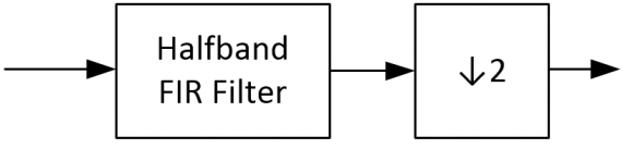
After the halfband (anti-aliasing) filter, the frequency response is easy to define. However, after we decimate by 2 (discard every 2nd sample), the impulse response now varies as a function of the impulse's alignment in time.

For example, one impulse alignment might give an output something like this:

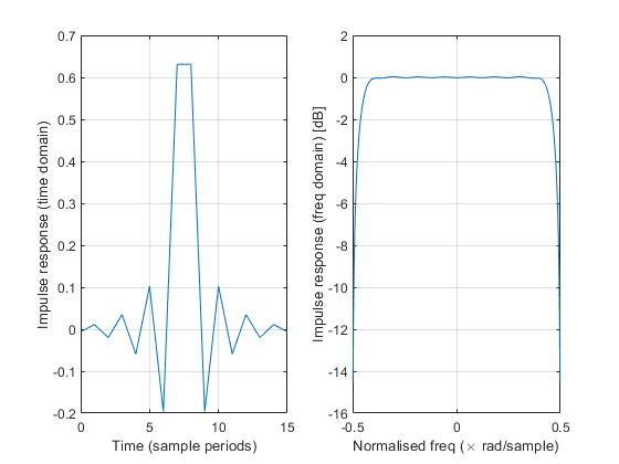
whereas offsetting the input impulse by +/- 1 sample would give an output like this:

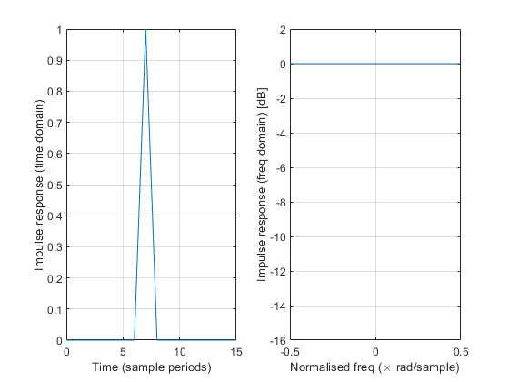
(because in this alignment, we retain only the centre tap and all the zero-valued taps in the halfband filter).

I have a vague and distant memory telling me this could possibly mean that this decimator is not Linear Time Invariant, so the impulse response doesn't completely characterise the system. Whether that's correct or not, I'm still left wondering how I can characterise this system. I don't think either of the spectra above are the answer (how would we even choose which one?).

As a next step, I was considering inputting a long stream of spectrally flat Gaussian noise and seeing what came out. However, I would then need an infinite number of samples (and an excellent noise source) to exactly characterise the system. Is there a better way?

You need to spiff up your memory, for sure.

Yes, the decimator is not linear time invariant (LTI).  That is because the sampling step is time-varying.  So it cannot be characterized by an impulse response that's only dependent on delay (i.e. $$h(\tau)$$).

The system is still linear, however, and that means that it can be characterized by an impulse response: it will just be one that is time dependent: $$h(\tau, t)$$, with $$\tau$$ being the delay.  Moreover, it'll be dependent on $$h(\tau, t \bmod N)$$, where N is the overall amount of decimation, so there's a finite number of terms in the impulse response.

(Someone please reply to this with the correct format for in-line mathjax -- I know there's a tutorial for this site that shows the proper escape sequenc, but I can't find it.  My apologies.)

If a system is not LTI, I'm a bit lost...

In the case of my example, if I make the approximation that the anti-aliasing filter's frequency response is zero outside the band of interest, then the decimation introduces no spectral wrapping... so I feel like it should be valid to just chop the sides off the original filter's frequency response, and that would fully characterise the system.

However, if I can't assume the response is exactly zero outside the band, then is there no single frequency response that can meaningfully characterise the system? If not, then what is the recommended way to proceed with analysis? (For example, if I want to ensure I won't exceed regulations for out-of-band emissions).

EDIT: I guess if the system is not LTI, then we can't use the traditional spectrum_in -> spectrum_out characterisation. For example, instead of inputting an impulse, I could input spectrally flat Gaussian noise (whose frequency spectrum has constant magnitude equal to that of the impulse).

Despite having the same input spectrum (magnitude) as the impulse, I would now expect the output spectra to be the same at any timing offset (because the odd and even samples have identical statistics). Indeed, simulating over a finite number of samples, the two spectra seem to be converging towards the same shape:

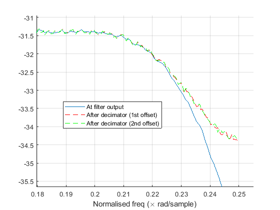
So, in this graph, I can see that the spectrum at the decimator output (for either timing offset) is well approximated by the spectrum at the filter output (at least for this particular input signal), EXCEPT near the edge of the band, where we can see extra residuals from spectral wrapping.

I think my question is about whether we can characterise/analyse these imperfections without resorting to large-sample simulations. Perhaps I would need to enforce the assumption that the statistics of the input signal are identical for all timing offsets (but in my case, and perhaps many practical cases, I think this is a sound assumption).

Hi weetabixharry.

I don't understand the spectral curves or the "timing offset" topic of your recent reply, but I can say you are correct in that your multirate digital filter is not LTI. Because its input and output frequency ranges are different, your multirate digital filter does not have a z-domain transfer function nor a frequency response in the traditional sense. I discuss these ideas at:

https://www.dsprelated.com/showarticle/143.php

However, you certainly can characterize your multirate digital filter’s frequency-domain behavior. One way to do so is to apply a chirp signal (scanning a freq range from just above zero Hz to just below the decimating filter’s input Fs/2 Hz) to your multirate digital filter and plot the spectrum of the filter’s output. Make the time duration of the chirp signal, say, P = 10 times the group delay of your filter. (Experiment with different values of P.)

Another way to characterize your multirate digital filter’s frequency-domain behavior is to apply a wideband noise signal to your decimating filter and plot the spectrum of the filter’s output. Make the variance of the noise signal, say, Q = 10 times the variance quantization noise of your filter’s input data words. (Experiment with different values of Q.)

A third way to characterize your decimate-by-two digital filter’s frequency-domain behavior is the way the “professionals” do it. That is, apply a unit impulse signal to your lowpass filter (no decimation!) and compute the lowpass filter’s output signal spectrum. Next circularly rotate that complex-valued spectrum by half the input’s sample rate so that the original zero-Hz spectral component is now residing at Fs/2 Hz. Add that circularly rotated complex-valued spectrum to your original (unrotated) complex-valued spectrum. Then plot the magnitude of the summed spectrum.

Good Luck.

@Rick Lyons

Brilliant. Thank you for the excellent response. Your article looks like exactly what I was looking for from the start (if only I had entered better search terms into Google!). I look forward to reading through it properly today.

I think I can clarify what I was trying to say about the "timing offsets" in the context of your third ("professional") characterisation. One way of seeing why that method works is to view the decimation as a point-wise multiplication in the time domain by [1,0,1,0,1,0,...].

If I recall correctly, (point-wise) multiplication in the time/freq domain is equivalent to (circular) convolution in the freq/time domain. So, the decimation is equivalent to convolving the frequency response by FFT{[1,0,1,0,1,0,...]} = [N/2,0,0,0,0,0,0,...,N/2,0,0,0,0,0,0,...] (over N discrete points).

If I'm not wrong, then this convolution describes exactly the sum you described (up to a scaling factor).

However, if we instead decimate in the second alignment: [0,1,0,1,0,1,...], then the equivalent freq-domain convolution amounts to subtracting the shifted spectrum instead of adding. This is the difference between the two sets of graphs in my original post (and between the green and red plots in my second post).

EDIT: Multiplying by [1,0,1,0,...] doesn't actually describe the act of discarding samples (changing the rate), but there still seems to be some merit in looking at it this way.

I can look at the dn2 as having three outputs! the full stream before decimation then the decimated stream1 that discards every odd sample and decimated stream2 that discards every even sample. For the full stream the dn2 response must have done its job and removed any frequencies that would alias after decimation. Once that condition fulfilled then selecting either odd or even streams should result in same output in frequency domain with one sample delay difference relative to input rate. The two streams can be thought of as same "analogue" signal sampled with phase shift at an ADC. For delay issues I can't depend on a single impulse input as it could end up in the odd stream or the even. But impulse input is ok for modelling through from input to output.

I can also characterize group delay and frequency response on the full stream then see effect of final odd/even selection. This odd/even becomes implementation issue.

Hi,

Take a look at my post on this subject:

https://www.dsprelated.com/showarticle/1228.php

regards,

Neil

@neirober

Great, thanks Neil. I am amazed (and a little embarrassed) that I didn't find your post in any of my Google searches.

This looks like really valuable material and I look forward to working through it today.

I read through your post quickly and, if I understand correctly, you are saying that the multi-stage decimator is still equivalent if we reorder the filtering and decimating (as long as we account for the changed rates by upsampling the filter taps).

If that's true, then that's a pretty remarkable (and powerful) result - and one that wouldn't be immediately obvious to me. I feel I need to run through some examples in MATLAB to convince myself that the spectral wrapping residuals from each stage behave the same in the equivalent model. I'll post back here with some comments after that.

As I'm writing this, a very faint memory is floating through my mind of a bespectacled lecturer saying something about "Noble identities", which I have a feeling could be relevant here. Instead of listening carefully, I recall wondering whether these identities were supposed to exhibit high moral principles, or whether they were just invented by some guy called Mr. Noble.

Weetabixharry,

I'm not saying to reorder the filtering and downsampling -- If you look at figure 5, what I am doing is cascading versions of each filter that are sampled at fs.  This requires upsampling b2 and b3.

regards,

Neil

I summarize this process on page 6 of the pdf version.

@neirober

I could be misunderstanding, but there may also be different (equally valid) ways to look at it. In the summary, I see Steps 1 and 2 as moving all the FIR boxes in Figure 1 to the left. (Convolving the three impulse responses is equivalent to applying the three FIR filters consecutively in series, having compensated for rate changes in Step 1).

Then, I view the "Taking aliasing into account" section as doing all of the decimation in one go (i.e. we moved all the down-arrow boxes in Figure 1 to the right, and combined them into one down-by-8 box).

As I said before, it's not immediately clear to me that this is exactly equivalent in a general sense. However, those "Noble Identities" I mentioned seem to suggest that it is:

https://www.dsprelated.com/freebooks/sasp/Multirat...

EDIT: I ran a really quick test in MATLAB and this does work. You can basically move the FIR boxes left and every time time you hop over a down-arrow box, you just need to upsample the taps by that amount. This is hugely helpful in my analysis.

Yes, that's right.

Neil