Constant Peak-Gain Resonator

Free Books Introduction to Digital Filters

It is surprisingly easy to normalize exactly the peak gain in a second-order resonator tuned by a single coefficient [94]. The filter structure that accomplishes this is the one we already considered in §B.6.1:

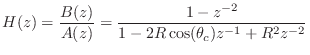
$\displaystyle H(z) = \frac{B(z)}{A(z)} = \frac{1 - z^{-2}}{1-2R\cos(\theta_c)z^{-1}+ R^2z^{-2}}$

(B.14)

That is, the two-pole resonator normalized by zeros at $z=\pm 1$ has the constant peak-gain property when it has resonant peaks in its response at all. Note, however, that the peak-gain frequency and the pole-resonance frequency (cf. §B.6.3), are generally two different things, as elaborated below. This structure has the added bonus that its difference equation requires only one more addition relative to the unnormalized two-pole resonator, and no new multiply.

Real-time audio ``plugins'' based on the constant-peak-gain resonator are developed in Appendix K.

The peak gain is , so multiplying the transfer function by normalizes the peak gain to one for all tunings. It can also be shown [94] that the peak gain coincides with the variance gain when the resonator is driven by white noise. That is, if the variance of the driving noise is $\sigma^2$ , the variance of the noise at the resonator output is $2\sigma^2/(1-R^2)$ . Therefore, scaling the resonator input by $g=\sqrt{(1-R^2)/2}$ will normalize the resonator such that the output signal power equals the input signal power when the input signal is white noise.

Frequency response overlays for the constant-peak-gain resonator are shown in Fig.B.23 (), Fig.B.20 (), and Fig.B.21 (). While the peak frequency may be far from the resonance tuning in the more heavily damped examples, the peak gain is always normalized to unity. The normalized radian frequency $\psi\in[-\pi,\pi]$ at which the peak gain occurs is related to the pole angle $\theta_c\in[-\pi,\pi]$ by [94]

$\displaystyle \cos(\theta_c) = \frac{1+R^2}{2R}\cos(\psi). \protect$

(B.15)

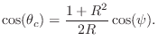
When the right-hand side of the above equation exceeds 1 in magnitude, there is no (real) solution for the pole frequency $\theta _c$ . This happens, for example, when

is less than 1 and $\psi$ is too close to 0 or $\pi$ . Conversely, given any pole angle $\theta_c\in(0,\pi)$ , there always exists a solution for the peak frequency $\psi = \arccos[2R\cos(\omega_c)/(1+R^2)]$ , since $\vert 2R/(1+R^2)\vert\leq1$ when $R\in[0,1]$ . However, when

is small, the peak frequency can be far from the pole resonance frequency, as shown in Fig.B.22.

**Figure B.22:** Upper and lower peak-gain frequency limits as a function of pole radius ( $\arccos[\pm2R/(1+R^2)]$ ).
$\includegraphics[width=\twidth ]{eps/psivsthetac}$

Thus, must be close to 1 to obtain a resonant peak near dc (a case commonly needed in audio work) or half the sampling rate (rarely needed in practice). When is much less than 1, the peak frequency $\psi$ cannot leave a small interval near one-fourth the sampling rate, as can be seen at the far left in Fig.B.22.

Figure B.22 predicts that for , the lowest peak-gain frequency should be around $\psi\geq 0.515$ radian per sample. Figure B.21 agrees with this prediction.

As Figures B.23 through B.25 show, the peak gain remains constant even at very low and very high frequencies, to the extent they are reachable for a given . The zeros at dc and preclude the possibility of peaks at exactly those frequencies, but for near 1, we can get very close to having a peak at dc or , as shown in Figures B.19 and B.20.