


Conical Acoustic Tubes
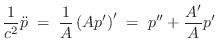
The conical acoustic tube is a one-dimensional waveguide which propagates circular sections of spherical pressure waves in place of the plane wave which traverses a cylindrical acoustic tube [22,349]. The wave equation in the spherically symmetric case is given by
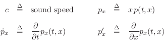
where
Spherical coordinates are appropriate because simple closed-form
solutions to the wave equation are only possible when the forced boundary
conditions lie along coordinate planes. In the case of a cone, the
boundary conditions lie along a conical section of a sphere. It can be
seen that the wave equation in a cone is identical to the wave equation in
a cylinder, except that ![]() is replaced by
is replaced by ![]() . Thus, the solution is a
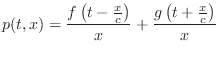
superposition of left- and right-going traveling wave components, scaled by
. Thus, the solution is a
superposition of left- and right-going traveling wave components, scaled by
![]() :
:
where
In cylindrical tubes, the velocity wave is in phase with the pressure wave. This is not the case with conical or more general tubes. The velocity of a traveling may be computed from the corresponding traveling pressure wave by dividing by the wave impedance.
Digital Simulation
A discrete-time simulation of the above solution may be obtained by simply
sampling the traveling-wave amplitude at intervals of ![]() seconds, which implies a spatial sampling interval of
seconds, which implies a spatial sampling interval of
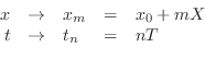
![]() meters. Sampling is carried out mathematically by the
change of variables
meters. Sampling is carried out mathematically by the
change of variables
![\begin{eqnarray*}
x_mp(t_n,x_m) &\,\mathrel{\mathop=}\,& f(t_n- x_m/c)+g(t_n+ x...
...hop=}\,& f\left[(n-m)T-x_0/c\right]+ g\left[(n+m)T+x_0/c\right].
\end{eqnarray*}](http://www.dsprelated.com/josimages_new/pasp/img4258.png)
Define
![\includegraphics[width=\twidth]{eps/fcideal}](http://www.dsprelated.com/josimages_new/pasp/img4261.png) |
A more compact simulation diagram which stands for either sampled or continuous simulation is shown in Figure C.44. The figure emphasizes that the ideal, lossless waveguide is simulated by a bidirectional delay line.
![\includegraphics[width=\twidth]{eps/fcone}](http://www.dsprelated.com/josimages_new/pasp/img4262.png)
As in the case of uniform waveguides, the digital simulation of the traveling-wave solution to the lossless wave equation in spherical coordinates is exact at the sampling instants, to within numerical precision, provided that the traveling waveshapes are initially bandlimited to less than half the sampling frequency. Also as before, bandlimited interpolation can be used to provide time samples or position samples at points off the simulation grid. Extensions to include losses, such as air absorption and thermal conduction, or dispersion, can be carried out as described in §2.3 and §C.5 for plane-wave propagation (through a uniform wave impedance).
The simulation of Fig.C.44 suffices to simulate an isolated conical frustum, but what if we wish to interconnect two or more conical bores? Even more importantly, what driving-point impedance does a mouthpiece ``see'' when attached to the narrow end of a conical bore? The preceding only considered pressure-wave behavior. We must now also find the velocity wave, and form their ratio to obtain the driving-point impedance of a conical tube.
Next Section:
Momentum Conservation in Nonuniform Tubes
Previous Section:
Horns as Waveguides


