


Finite Difference Approximation vs. Bilinear Transform
Recall that the Finite Difference Approximation (FDA) defines the
elementary differentiator by
![]() (ignoring the
scale factor
(ignoring the
scale factor ![]() for now), and this approximates the ideal transfer
function
for now), and this approximates the ideal transfer
function ![]() by
by
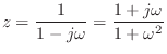
![]() . The bilinear transform
calls instead for the transfer function
. The bilinear transform
calls instead for the transfer function
![]() (again
dropping the scale factor) which introduces a pole at
(again
dropping the scale factor) which introduces a pole at ![]() and gives
us the recursion
and gives
us the recursion
![]() .
Note that this new pole is right on the unit circle and is therefore
undamped. Any signal energy at half the sampling rate will circulate
forever in the recursion, and due to round-off error, it will tend to
grow. This is therefore a potentially problematic revision of the
differentiator. To get something more practical, we need to specify
that the filter frequency response approximate
.
Note that this new pole is right on the unit circle and is therefore
undamped. Any signal energy at half the sampling rate will circulate
forever in the recursion, and due to round-off error, it will tend to
grow. This is therefore a potentially problematic revision of the
differentiator. To get something more practical, we need to specify
that the filter frequency response approximate
![]() over a
finite range of frequencies
over a
finite range of frequencies
![]() , where
, where
![]() , above which we allow the response to ``roll off''
to zero. This is how we pose the differentiator problem in terms of
general purpose filter design (see §8.6) [362].
, above which we allow the response to ``roll off''
to zero. This is how we pose the differentiator problem in terms of
general purpose filter design (see §8.6) [362].
To understand the properties of the finite difference approximation in the
frequency domain, we may look at the properties of its ![]() -plane
to
-plane
to ![]() -plane mapping
-plane mapping

Setting ![]() to 1 for simplicity and solving the FDA mapping for z gives
to 1 for simplicity and solving the FDA mapping for z gives
![\includegraphics[width=3in]{eps/lfdacirc}](http://www.dsprelated.com/josimages_new/pasp/img1678.png)
Under the FDA, analog and digital frequency axes coincide well enough at
very low frequencies (high sampling rates), but at high frequencies
relative to the sampling rate, artificial damping is introduced as
the image of the ![]() axis diverges away from the unit circle.
axis diverges away from the unit circle.
While the bilinear transform ``warps'' the frequency axis, we can say the FDA ``doubly warps'' the frequency axis: It has a progressive, compressive warping in the direction of increasing frequency, like the bilinear transform, but unlike the bilinear transform, it also warps normal to the frequency axis.
Consider a point traversing the upper half of the unit circle in the z
plane, starting at ![]() and ending at
and ending at ![]() . At dc, the FDA is
perfect, but as we proceed out along the unit circle, we diverge from the
. At dc, the FDA is
perfect, but as we proceed out along the unit circle, we diverge from the
![]() axis image and carve an arc somewhere out in the image of the
right-half
axis image and carve an arc somewhere out in the image of the
right-half ![]() plane. This has the effect of introducing an artificial
damping.
plane. This has the effect of introducing an artificial
damping.
Consider, for example, an undamped mass-spring system. There will be a
complex conjugate pair of poles on the ![]() axis in the
axis in the ![]() plane. After
the FDA, those poles will be inside the unit circle, and therefore damped
in the digital counterpart. The higher the resonance frequency, the larger
the damping. It is even possible for unstable
plane. After
the FDA, those poles will be inside the unit circle, and therefore damped
in the digital counterpart. The higher the resonance frequency, the larger
the damping. It is even possible for unstable ![]() -plane poles to be mapped
to stable
-plane poles to be mapped
to stable ![]() -plane poles.
-plane poles.
In summary, both the bilinear transform and the FDA preserve order,
stability, and positive realness. They are both free of aliasing, high
frequencies are compressively warped, and both become ideal at dc, or as
![]() approaches
approaches ![]() . However, at frequencies significantly above
zero relative to the sampling rate, only the FDA introduces artificial
damping. The bilinear transform maps the continuous-time frequency axis in
the
. However, at frequencies significantly above
zero relative to the sampling rate, only the FDA introduces artificial
damping. The bilinear transform maps the continuous-time frequency axis in
the ![]() (the
(the ![]() axis) plane precisely to the discrete-time frequency
axis in the
axis) plane precisely to the discrete-time frequency
axis in the ![]() plane (the unit circle).
plane (the unit circle).
Next Section:
Practical Considerations
Previous Section:
Delay Operator Notation


