


First-Order Delay-Filter Design
The first-order case is very simple while enabling separate control of
low-frequency and high-frequency reverberation times. For simplicity,
let's specify ![]() and
and
![]() , denoting the desired
decay-time at dc (
, denoting the desired
decay-time at dc (![]() ) and half the sampling rate
(
) and half the sampling rate
(
![]() ). Then we have determined the coefficients of a
one-pole filter:
). Then we have determined the coefficients of a
one-pole filter:
![\begin{eqnarray*}
\frac{g_i}{1-p_i} &=& 10^{-3 M_i T / t_{60}(0)}
\eqsp e^{-M_iT...
...(\pi/T)}
\eqsp e^{-M_iT/\tau(\pi/T)} \isdefs R_\pi^{M_i}\\ [5pt]
\end{eqnarray*}](http://www.dsprelated.com/josimages_new/pasp/img870.png)
where
![]() denotes the
denotes the ![]() th delay-line length in
seconds. These two equations are readily solved to yield
th delay-line length in
seconds. These two equations are readily solved to yield
![\begin{eqnarray*}
p_i &=& \frac{R_0^{M_i}-R_\pi^{M_i}}{R_0^{M_i}+R_\pi^{M_i}}\\ [5pt]
g_i &=& \frac{2R_0^{M_i}R_\pi^{M_i}}{R_0^{M_i}+R_\pi^{M_i}}
\end{eqnarray*}](http://www.dsprelated.com/josimages_new/pasp/img872.png)
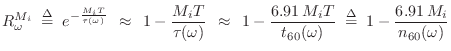
The truncated series approximation
Next Section:
Orthogonalized First-Order Delay-Filter Design
Previous Section:
Damping Filters for Reverberation Delay Lines


