


Window Design by Linear Programming
This section, based on a class project by EE graduate student Tatsuki Kashitani, illustrates the use of linprog in Matlab for designing variations on the Chebyshev window (§3.10). In addition, some comparisons between standard linear programming and the Remez exchange algorithm (firpm) are noted.
Linear Programming (LP)
If we can get our filter or window design problems in the form
![\begin{displaymath}\begin{array}[t]{ll} \mathrm{minimize} & f^{T}x\\ \mathrm{subject}\, \mathrm{to} & \begin{array}[t]{l} \mathbf{A}_{eq}x=b_{eq}\\ \mathbf{A}x\le b\end{array}, \end{array}\end{displaymath}](http://www.dsprelated.com/josimages_new/sasp2/img581.png) |
(4.60) |
where
The linprog function in Matlab Optimization Toolbox solves LP problems. In Octave, one can use glpk instead (from the GNU GLPK library).
LP Formulation of Chebyshev Window Design
What we want:
- Symmetric zero-phase window.
- Window samples to be positive.
(4.61)
- Transform to be 1 at DC.

(4.62)
- Transform to be within
![$ \left[-\delta ,\delta \right]$](http://www.dsprelated.com/josimages_new/sasp2/img588.png) in the stop-band.
in the stop-band.
(4.63)
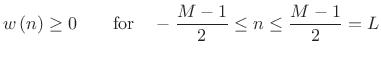
- And
 to be small.
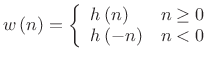
Symmetric Window Constraint
Because we are designing a zero-phase window, use only the
positive-time part
![]() :
:
| (4.64) |
 |
(4.65) |
Positive Window-Sample Constraint
For each window sample,
![]() , or,
, or,
| (4.66) |
Stacking inequalities for all
![$\displaystyle \left[\begin{array}{ccccc} -1 & 0 & \cdots & 0 & 0\\ 0 & -1 & & & 0\\ \vdots & & \ddots & & \vdots \\ 0 & & & -1 & 0\\ 0 & 0 & \cdots & 0 & -1\end{array} \right]\left[\begin{array}{c} h\left(0\right)\\ h\left(1\right)\\ \vdots \\ h\left(L-1\right)\\ h\left(L\right)\end{array} \right] \le \left[\begin{array}{c} 0\\ 0\\ \vdots \\ 0\\ 0 \end{array} \right]$](http://www.dsprelated.com/josimages_new/sasp2/img596.png) |
(4.67) |
or
| (4.68) |
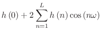
DC Constraint
The DTFT at frequency ![]() is given by
is given by
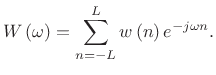 |
(4.69) |
By zero-phase symmetry,
 |
|||
![$\displaystyle \left[\begin{array}{cccc}
1 & 2\cos \left(\omega \right) & \cdots & 2\cos \left(L\omega \right)\end{array}\right]\left[\begin{array}{c}
h\left(0\right)\\
h\left(1\right)\\
\vdots \\
h\left(L\right)\end{array}\right]$](http://www.dsprelated.com/josimages_new/sasp2/img601.png) |
|||
So
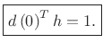 |
(4.70) |
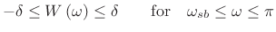
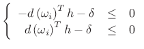
Sidelobe Specification
Likewise, side-lobe specification can be enforced at frequencies
![]() in the stop-band.
in the stop-band.
| (4.71) |
or
 |
(4.72) |
where
| (4.73) |
We need
![$\displaystyle \left[\begin{array}{c}
-d\left(\omega _1\right)^{T}\\
\vdots \\
-d\left(\omega _{K}\right)^{T}\\
d\left(\omega _1\right)^{T}\\
\vdots \\
d\left(\omega _{K}\right)^{T}\end{array}\right]h+\left[\begin{array}{c}
-\delta \\
\vdots \\
-\delta \\
-\delta \\
\vdots \\
-\delta \end{array}\right]$](http://www.dsprelated.com/josimages_new/sasp2/img610.png) |
|||
![$\displaystyle \left[\begin{array}{cc}
-d\left(\omega _1\right)^{T} & -1\\
\vdots & \vdots \\
-d\left(\omega _{K}\right)^{T} & -1\\
d\left(\omega _1\right)^{T} & -1\\
\vdots & \vdots \\
d\left(\omega _{K}\right)^{T} & -1
\end{array}\right]\left[\begin{array}{c}
h\\
\delta \end{array}\right]$](http://www.dsprelated.com/josimages_new/sasp2/img613.png) |
I.e.,
![$\displaystyle \zbox {\mathbf{A}_{sb}\left[\begin{array}{c} h\\ \delta \end{array} \right] \le \mathbf{0}.}$](http://www.dsprelated.com/josimages_new/sasp2/img615.png) |
(4.74) |
LP Standard Form
Now gather all of the constraints to form an LP problem:
![\begin{displaymath}\begin{array}[t]{ll} \mathrm{minimize} & \left[\begin{array}{cccc} 0 & \cdots & 0 & 1\end{array} \right] \left[\begin{array}{c} h\\ \delta \end{array} \right]\\ [5pt] \mbox{subject to} & \begin{array}[t]{l} \left[\begin{array}{cc} d\left(0\right)^{T} & 0\end{array} \right]\left[\begin{array}{c} h\\ \delta \end{array} \right]=1\\ \left[\begin{array}{c} \left[\begin{array}{cc} -\mathbf{I} & \mathbf{0}\end{array} \right]\\ [5pt] \mathbf{A}_{sb}\end{array} \right]\left[\begin{array}{c} h\\ \delta \end{array} \right]\le \mathbf{0}\end{array} \end{array}\end{displaymath}](http://www.dsprelated.com/josimages_new/sasp2/img616.png) |
(4.75) |
where the optimization variables are
Solving this linear-programming problem should produce a window that is optimal in the Chebyshev sense over the chosen frequency samples, as shown in Fig.3.37. If the chosen frequency samples happen to include all of the extremal frequencies (frequencies of maximum error in the DTFT of the window), then the unique Chebyshev window for the specified main-lobe width must be obtained. Iterating to find the extremal frequencies is the heart of the Remez multiple exchange algorithm, discussed in the next section.
![\includegraphics[width=\twidth,height=6.5in]{eps/print_normal_chebwin}](http://www.dsprelated.com/josimages_new/sasp2/img618.png)
Remez Exchange Algorithm
The Remez multiple exchange algorithm works by moving the frequency samples each iteration to points of maximum error (on a denser grid). Remez iterations could be added to our formulation as well. The Remez multiple exchange algorithm (function firpm [formerly remez] in the Matlab Signal Processing Toolbox, and still remez in Octave) is normally faster than a linear programming formulation, which can be regarded as a single exchange method [224, p. 140]. Another reason for the speed of firpm is that it solves the following equations non-iteratively for the filter exhibiting the desired error alternation over the current set of extremal frequencies:
![$\displaystyle \left[ \begin{array}{c} H(\omega_1) \\ H(\omega_2) \\ \vdots \\ H(\omega_{K}) \end{array} \right] = \left[ \begin{array}{cccccc} 1 & 2\cos(\omega_1) & \dots & 2\cos(\omega_1L) & \frac{1}{W(\omega_1)} \\ 1 & 2\cos(\omega_2) & \dots & 2\cos(\omega_2L) & \frac{-1}{W(\omega_2)} \\ \vdots & & & \\ 1 & 2\cos(\omega_{K}) & \dots & 2\cos(\omega_{K}L) & \frac{(-1)^{K}}{W(\omega_{K})} \end{array} \right] \left[ \begin{array}{c} h_0 \\ h_1 \\ \vdots \\ h_{L} \\ \delta \end{array} \right]$](http://www.dsprelated.com/josimages_new/sasp2/img619.png) |
(4.76) |
where
Convergence of Remez Exchange
According to a theorem of Remez, ![]() is guaranteed to
increase monotonically each iteration, ultimately converging to
its optimal value. This value is reached when all the extremal
frequencies are found. In practice, numerical round-off error may
cause
is guaranteed to
increase monotonically each iteration, ultimately converging to
its optimal value. This value is reached when all the extremal
frequencies are found. In practice, numerical round-off error may
cause ![]() not to increase monotonically. When this is detected,
the algorithm normally halts and reports a failure to converge.
Convergence failure is common in practice for FIR filters having more
than 300 or so taps and stringent design specifications (such as very
narrow pass-bands). Further details on Remez exchange are given
in [224, p. 136].
not to increase monotonically. When this is detected,
the algorithm normally halts and reports a failure to converge.
Convergence failure is common in practice for FIR filters having more
than 300 or so taps and stringent design specifications (such as very
narrow pass-bands). Further details on Remez exchange are given
in [224, p. 136].
As a result of the non-iterative internal LP solution on each iteration, firpm cannot be used when additional constraints are added, such as those to be discussed in the following sections. In such cases, a more general LP solver such as linprog must be used. Recent advances in convex optimization enable faster solution of much larger problems [22].
Monotonicity Constraint
We can constrain the positive-time part of the window to be monotonically decreasing:
| (4.77) |
In matrix form,
![$\displaystyle \left[\begin{array}{ccccc}
-1 & 1 & & & 0\\
& -1 & 1 & & \\
& & \ddots & \ddots & \\
0 & & & -1 & 1\end{array}\right]h$](http://www.dsprelated.com/josimages_new/sasp2/img623.png) |
or,
| (4.78) |
See Fig.3.38.
![\includegraphics[width=\twidth,height=6.5in]{eps/print_monotonic_chebwin}](http://www.dsprelated.com/josimages_new/sasp2/img626.png)
L-Infinity Norm of Derivative Objective
We can add a smoothness objective by adding
![]() -norm of the
derivative to the objective function.
-norm of the
derivative to the objective function.
| (4.79) |
The
![]() -norm only cares about the maximum derivative.
Large
-norm only cares about the maximum derivative.
Large ![]() means we put more weight on the smoothness than the
side-lobe level.
means we put more weight on the smoothness than the
side-lobe level.
This can be formulated as an LP by adding one optimization parameter
![]() which bounds all derivatives.
which bounds all derivatives.
| (4.80) |
In matrix form,
![$\displaystyle \left[\begin{array}{r}
-\mathbf{D}\\
\mathbf{D}\end{array}\right]h-\sigma \mathbf1$](http://www.dsprelated.com/josimages_new/sasp2/img631.png) |
Objective function becomes
| (4.81) |
The result of adding the Chebyshev norm of diff(h) to the
objective function to be minimized (![]() ) is shown in
Fig.3.39. The result of increasing
) is shown in
Fig.3.39. The result of increasing ![]() to 20 is
shown in Fig.3.40.
to 20 is
shown in Fig.3.40.
![\includegraphics[width=\twidth,height=6.5in]{eps/print_linf_chebwin_1}](http://www.dsprelated.com/josimages_new/sasp2/img634.png)
![\includegraphics[width=\twidth,height=6.5in]{eps/print_linf_chebwin_2}](http://www.dsprelated.com/josimages_new/sasp2/img635.png)
L-One Norm of Derivative Objective
Another way to add smoothness constraint is to add ![]() -norm of
the derivative to the objective:
-norm of
the derivative to the objective:
| (4.82) |
Note that the
We can formulate an LP problem by adding a vector of optimization
parameters ![]() which bound derivatives:
which bound derivatives:
| (4.83) |
In matrix form,
![$\displaystyle \left[\begin{array}{r} -\mathbf{D}\\ \mathbf{D}\end{array} \right]h-\left[\begin{array}{c} -\tau \\ -\tau \end{array} \right]\le 0.$](http://www.dsprelated.com/josimages_new/sasp2/img638.png) |
(4.84) |
The objective function becomes
| (4.85) |
See Fig.3.41 and Fig.3.42 for example results.
![\includegraphics[width=\twidth,height=6.5in]{eps/print_lone_chebwin_1}](http://www.dsprelated.com/josimages_new/sasp2/img640.png)
![\includegraphics[width=\twidth,height=6.5in]{eps/print_lone_chebwin_2}](http://www.dsprelated.com/josimages_new/sasp2/img641.png)
Summary
This section illustrated the design of optimal spectrum-analysis windows made using linear-programming (linprog in matlab) or Remez multiple exchange algorithms (firpm in Matlab). After formulating the Chebyshev window as a linear programming problem, we found we could impose a monotonicity constraint on its shape in the time domain, or various derivative constraints. In Chapter 4, we will look at methods for FIR filter design, including the window method (§4.5) which designs FIR filters as a windowed ideal impulse response. The formulation introduced in this section can be used to design such windows, and it can be used to design optimal FIR filters. In such cases, the impulse response is designed directly (as the window was here) to minimize an error criterion subject to various equality and inequality constraints, as discussed above for window design.4.16
Next Section:
The Ideal Lowpass Filter
Previous Section:
Optimized Windows


