


Window Method for FIR Filter Design
The window method for digital filter design is fast, convenient, and robust, but generally suboptimal. It is easily understood in terms of the convolution theorem for Fourier transforms, making it instructive to study after the Fourier theorems and windows for spectrum analysis. It can be effectively combined with the frequency sampling method, as we will see in §4.6 below.
The window method consists of simply ``windowing'' a theoretically
ideal filter impulse response ![]() by some suitably chosen window
function
by some suitably chosen window
function ![]() , yielding
, yielding
| (5.8) |
For example, as derived in Eq.
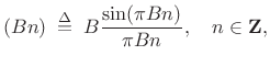 |
(5.9) |
where
Since
![]() sinc
sinc![]() decays away from time 0 as
decays away from time 0 as ![]() , we would
expect to be able to truncate it to the interval
, we would
expect to be able to truncate it to the interval ![]() , for some
sufficiently large
, for some
sufficiently large ![]() , and obtain a pretty good FIR filter which
approximates the ideal filter. This would be an example of using the
window method with the rectangular window. We saw in
§4.3 that such a choice is optimal in the least-squares
sense, but it designs relatively poor audio filters. Choosing other
windows corresponds to tapering the ideal impulse response to
zero instead of truncating it. Tapering better preserves the shape of
the desired frequency response, as we will see. By choosing the
window carefully, we can manage various trade-offs so as to maximize
the filter-design quality in a given application.
, and obtain a pretty good FIR filter which
approximates the ideal filter. This would be an example of using the
window method with the rectangular window. We saw in
§4.3 that such a choice is optimal in the least-squares
sense, but it designs relatively poor audio filters. Choosing other
windows corresponds to tapering the ideal impulse response to
zero instead of truncating it. Tapering better preserves the shape of
the desired frequency response, as we will see. By choosing the
window carefully, we can manage various trade-offs so as to maximize
the filter-design quality in a given application.
Window functions are always time limited. This means there is
always a finite integer ![]() such that
such that ![]() for all
for all
![]() . The final windowed impulse response
. The final windowed impulse response
![]() is thus always time-limited, as needed for practical
implementation. The window method always designs a
finite-impulse-response (FIR) digital filter (as opposed to an
infinite-impulse-response (IIR) digital filter).
is thus always time-limited, as needed for practical
implementation. The window method always designs a
finite-impulse-response (FIR) digital filter (as opposed to an
infinite-impulse-response (IIR) digital filter).
By the dual of the convolution theorem, pointwise multiplication in
the time domain corresponds to convolution in the frequency domain.
Thus, the designed filter ![]() has a frequency response given by
has a frequency response given by
| (5.10) |
where
- The pass-band gain is primarily the area under the
main lobe of the window transform, provided the main lobe
``fits'' inside the pass-band (i.e., the total lowpass bandwidth
 is greater than or equal to the main-lobe width
of
is greater than or equal to the main-lobe width
of  ).
).
- The stop-band gain is given by an integral over a portion
of the side lobes of the window transform. Since side-lobes
oscillate about zero, a finite integral over them is normally much
smaller than the side-lobes themselves, due to adjacent side-lobe
cancellation under the integral.
- The best stop-band performance occurs when the cut-off
frequency is set so that the stop-band side-lobe integral traverses a
whole number of side lobes.
- The transition bandwidth is equal to the bandwidth of
the main lobe of the window transform, again provided that the main
lobe ``fits'' inside the pass-band.
- For very small lowpass bandwidths
 ,
,  approaches an
impulse in the frequency domain. Since the impulse is the
identity operator under convolution, the resulting lowpass filter
approaches an
impulse in the frequency domain. Since the impulse is the
identity operator under convolution, the resulting lowpass filter
 approaches the window transform
  for small
. In particular, the stop-band gain approaches the window
side-lobe level, and the transition width approaches half the
main-lobe width. Thus, for good results, the lowpass cut-off
frequency should be set no lower than half the window's main-lobe
width.
for small
. In particular, the stop-band gain approaches the window
side-lobe level, and the transition width approaches half the
main-lobe width. Thus, for good results, the lowpass cut-off
frequency should be set no lower than half the window's main-lobe
width.
Matlab Support for the Window Method
Octave and the Matlab Signal Processing Toolbox have two functions implementing the window method for FIR digital filter design:
- fir1 designs lowpass, highpass, bandpass, and
multi-bandpass filters.
- fir2 takes an arbitrary magnitude frequency response
specification.
Bandpass Filter Design Example
The matlab code below designs a bandpass filter which passes
frequencies between 4 kHz and 6 kHz, allowing transition bands from 3-4
kHz and 6-8 kHz (i.e., the stop-bands are 0-3 kHz and 8-10 kHz, when the
sampling rate is 20 kHz). The desired stop-band attenuation is 80 dB,
and the pass-band ripple is required to be no greater than 0.1 dB. For
these specifications, the function kaiserord returns a beta
value of
![]() and a window length of
and a window length of ![]() . These values
are passed to the function kaiser which computes the window
function itself. The ideal bandpass-filter impulse response is
computed in fir1, and the supplied Kaiser window is applied
to shorten it to length
. These values
are passed to the function kaiser which computes the window
function itself. The ideal bandpass-filter impulse response is
computed in fir1, and the supplied Kaiser window is applied
to shorten it to length ![]() .
.
fs = 20000;                 % sampling rate
F = [3000 4000 6000 8000];  % band limits
A = [0 1 0];                % band type: 0='stop', 1='pass'
dev = [0.0001 10^(0.1/20)-1 0.0001]; % ripple/attenuation spec
[M,Wn,beta,typ] = kaiserord(F,A,dev,fs);  % window parameters
b = fir1(M,Wn,typ,kaiser(M+1,beta),'noscale'); % filter design
Note the conciseness of the matlab code thanks to the use of kaiserord and fir1 from Octave or the Matlab Signal Processing Toolbox.
Figure 4.6 shows the magnitude frequency response
![]() of the resulting FIR filter
of the resulting FIR filter ![]() . Note that
the upper pass-band edge has been moved to 6500 Hz instead of 6000 Hz,
and the stop-band begins at 7500 Hz instead of 8000 Hz as requested.
While this may look like a bug at first, it's actually a perfectly
fine solution. As discussed earlier (§4.5), all
transition-widths in filters designed by the window method must equal
the window-transform's main-lobe width. Therefore, the only way to
achieve specs when there are multiple transition regions specified is
to set the main-lobe width to the minimum transition width.
For the others, it makes sense to center the transition within
the requested transition region.
. Note that
the upper pass-band edge has been moved to 6500 Hz instead of 6000 Hz,
and the stop-band begins at 7500 Hz instead of 8000 Hz as requested.
While this may look like a bug at first, it's actually a perfectly
fine solution. As discussed earlier (§4.5), all
transition-widths in filters designed by the window method must equal
the window-transform's main-lobe width. Therefore, the only way to
achieve specs when there are multiple transition regions specified is
to set the main-lobe width to the minimum transition width.
For the others, it makes sense to center the transition within
the requested transition region.
![\includegraphics[width=\twidth]{eps/fltDesign}](http://www.dsprelated.com/josimages_new/sasp2/img724.png)
Under the Hood of kaiserord
Without kaiserord, we would need to implement Kaiser's
formula [115,67] for estimating the Kaiser-window
![]() required to achieve the given filter specs:
required to achieve the given filter specs:
![$\displaystyle \beta = \left\{\begin{array}{ll} 0.1102(A-8.7), & A > 50 \\ [5pt] 0.5842(A-21)^{0.4} + 0.07886(A-21), & 21< A < 50 \\ [5pt] 0, & A < 21, \\ \end{array} \right. \protect$](http://www.dsprelated.com/josimages_new/sasp2/img725.png)
where
A similar function from [198] for window design (as opposed to filter design5.7) is
![$\displaystyle \beta = \left\{\begin{array}{ll} 0, & A<13.26 \\ [5pt] 0.76609(A-13.26)^{0.4} + 0.09834(A-13.26), & 13.26< A < 60 \\ [5pt] 0.12438*(A+6.3), & 60<A<120, \\ \end{array} \right. \protect$](http://www.dsprelated.com/josimages_new/sasp2/img728.png)
where now
Similarly, the filter order ![]() is estimated from stop-band
attenuation
is estimated from stop-band
attenuation ![]() and desired transition width
and desired transition width
![]() using the
empirical formula
using the
empirical formula
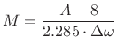 |
(5.13) |
where
Without the function fir1, we would have to manually
implement the window method of filter design by (1) constructing the
impulse response of the ideal bandpass filter ![]() (a cosine
modulated sinc function), (2) computing the Kaiser window
(a cosine
modulated sinc function), (2) computing the Kaiser window ![]() using
the estimated length and
using
the estimated length and ![]() from above, then finally (3)
windowing the ideal impulse response with the Kaiser window to obtain
the FIR filter coefficients
from above, then finally (3)
windowing the ideal impulse response with the Kaiser window to obtain
the FIR filter coefficients
![]() . A manual design of
this nature will be illustrated in the Hilbert transform example of
§4.6.
. A manual design of
this nature will be illustrated in the Hilbert transform example of
§4.6.
Comparison to the Optimal Chebyshev FIR Bandpass Filter
To provide some perspective on the results, let's compare the window method to the optimal Chebyshev FIR filter (§4.10) for the same length and design specifications above.
The following Matlab code illustrates two different bandpass filter designs. The first (different transition bands) illustrates a problem we'll look at. The second (equal transition bands, commented out), avoids the problem.
M = 101;
normF = [0 0.3 0.4 0.6 0.8 1.0];  % transition bands different
%normF = [0 0.3 0.4 0.6 0.7 1.0]; % transition bands the same
amp = [0 0 1 1 0 0];              % desired amplitude in each band

[b2,err2] = firpm(M-1,normF,amp); % optimal filter of length M
Figure 4.7 shows the frequency response of the Chebyshev FIR filter designed by firpm, to be compared with the window-method FIR filter in Fig.4.6. Note that the upper transition band ``blows up''. This is a well known failure mode in FIR filter design using the Remez exchange algorithm [176,224]. It can be eliminated by narrowing the transition band, as shown in Fig.4.8. There is no error penalty in the transition region, so it is necessary that each one be ``sufficiently narrow'' to avoid this phenomenon.
Remember the rule of thumb that the narrowest transition-band possible
for a length ![]() FIR filter is on the order of
FIR filter is on the order of ![]() , because
that's the width of the main-lobe of a length
, because
that's the width of the main-lobe of a length ![]() rectangular window
(measured between zero-crossings) (§3.1.2). Therefore, this
value is quite exact for the transition-widths of FIR bandpass filters
designed by the window method using the rectangular window (when the
main-lobe fits entirely within the adjacent pass-band and stop-band).
For a Hamming window, the window-method transition width would instead
be
rectangular window
(measured between zero-crossings) (§3.1.2). Therefore, this
value is quite exact for the transition-widths of FIR bandpass filters
designed by the window method using the rectangular window (when the
main-lobe fits entirely within the adjacent pass-band and stop-band).
For a Hamming window, the window-method transition width would instead
be ![]() . Thus, we might expect an optimal Chebyshev design to
provide transition widths in the vicinity of
. Thus, we might expect an optimal Chebyshev design to
provide transition widths in the vicinity of ![]() , but probably
not too close to
, but probably
not too close to ![]() or below
In the example above, where the sampling rate was
or below
In the example above, where the sampling rate was ![]() kHz, and the
filter length was
kHz, and the
filter length was ![]() , we expect to be able to achieve transition
bands circa
, we expect to be able to achieve transition
bands circa
![]() Hz, but not so low
as
Hz, but not so low
as
![]() Hz. As we found above,
Hz. As we found above,
![]() Hz was under-constrained, while
Hz was under-constrained, while ![]() Hz was ok, being near
the ``Hamming transition width.''
Hz was ok, being near
the ``Hamming transition width.''
![\includegraphics[width=\twidth]{eps/fltDesignRemez}](http://www.dsprelated.com/josimages_new/sasp2/img738.png) |
![\includegraphics[width=\twidth]{eps/fltDesignRemezTighter}](http://www.dsprelated.com/josimages_new/sasp2/img739.png) |
Next Section:
Hilbert Transform Design Example
Previous Section:
Frequency Sampling Method for FIR Filter Design


