


Phase or Frequency Shifter Using a Hilbert Transformer
In this article, we’ll describe how to use a Hilbert transformer to make a phase shifter or frequency shifter. In either case, the input is a real signal and the output is a real signal. We’ll use some simple Matlab code to simulate these systems. After that, we’ll go into a little more detail on Hilbert transformer theory and design.
Phase Shifter
A conceptual diagram of a phase shifter is shown in Figure 1, where the bold lines indicate complex signals. The input is cos(ωt+ϕ). As we’ll discuss later in this article, the Hilbert transformer [1,2] converts this input to a complex analytic signal ej(ωt+ϕ) = cos(ωt+ϕ) + jsin(ωt+ϕ). We multiply this signal by ejθ , where θ is the desired phase shift, to obtain the complex signal ej(ωt+ϕ+θ). The real part of this signal is our desired output: y= cos(ωt+ϕ+θ).
Writing the Hilbert complex output as I + jQ, y is then:
$$y= Re\{(I+jQ)e^{j\theta}\}$$
$$\qquad = Re\{(I+jQ)(cos\theta+jsin\theta\}$$
$$\qquad y= Icos\theta - Qsin\theta \qquad (1) $$
This allows us to implement the phase shifter using the block diagram of Figure 2. Note there is no “j” anywhere in Figure 2: all signals are real! In particular, the Q signal is a real number – in calculations we can use it to form the imaginary part of the complex signal I + jQ. As you probably know, I stands for In-phase component and Q stands for Quadrature component. I and Q are also frequently called xre and xim.
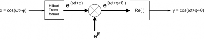
Figure 1.Phase Shifter Conceptual Diagram
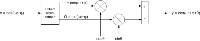
Figure 2. Phase Shifter Implementation.
The following Matlab code implements the block diagram of Figure 2. A 31-tap Hilbert transformer is realized as shown, where we take the theoretical coefficient values and multiply by a Hamming window to get the coefficients b1. We also create b2, which is a simple delay of 15 samples – this represents the delay of the center tap of the Hilbert transformer’s tapped delay network.
    % 31-tap Hilbert transformer
    b= 2/pi * [-1/15 0 -1/13 0 -1/11 0 -1/9 0 -1/7 0 -1/5 0 -1/3 0 -1 0 1 0 …
              1/3 0 1/5 0 1/7 0 1/9 0 1/11 0 1/13 0 1/15];
    b1= b.*hamming(31)';                          % window the coefficients
    b2= [0 0 0 0  0 0 0 0  0 0 0 0  0 0 0 1];     % delay of 15 (center tap of HT)
For a preview of the structure of the Hilbert transformer, see Figure 9. Next we create sinusoidal input x with frequency 6 Hz and sample frequency of 100 Hz:
    fs= 100;                    % Hz sample frequency
    Ts= 1/fs;
    N= 128;
    n= 0:N-1;
    f0= 6;                       % Hz freq of input signal
    x= cos(2*pi*f0*n*Ts);        % input signal
Now apply input x to the Hilbert transformer. The I output is just the center tap of the filter’s tapped delay line.
    I= filter(b2,1,x);        % I= center tap of HT
    Q= filter(b1,1,x);        % Q= output of HT
Finally, we implement equation 1 for phase shift of –π/3:
    theta= -pi/3;                          % rad phase shift with respect to I
    y= I*cos(theta) - Q*sin(theta);        % phase shifter output
Figures 1 and 2 assume no phase shift in the I-channel output of the Hilbert transformer. However, the actual implementation has a delay of 15 samples. This means the phase shift of –π/3 occurs with respect to the Hilbert transformer’s I output (center tap of the delay network). Figure 3 plots 32 samples of y and I on the same graph. As desired, y lags I by π/3 radians.
It’s worth noting that the phase shift does not depend on the frequency of the input sinusoid; as long as the frequency is within the passband of the Hilbert transformer, we get the desired phase shift. For example, Figure 4 shows a +π/4 phase shift for input signal frequencies of 6 Hz and 9 Hz.
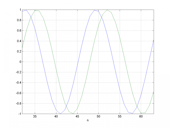
Figure 3.Phase Shifter input and output for f0 = 6 Hz, fs= 100 Hz, and ϕ= - π/3
Blue = Hilbert I-channel Green=output
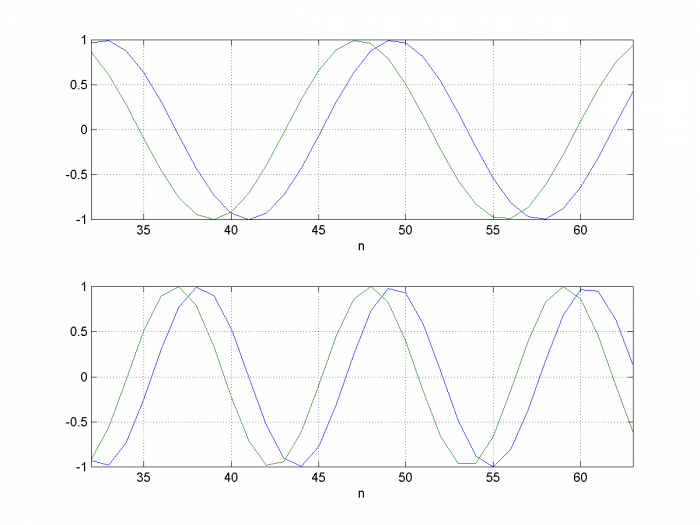
Figure 4.Phase Shifter I channel (blue) and output (green) for ϕ= + π/4, fs= 100 Hz.
Top: f0= 6 Hz Bottom: f0 = 9 Hz.
Frequency Shifter
The frequency shifter block diagram is shown in Figure 5. It is the same as the phase shifter, except we let θ in Equation 1 equal dω*t, where dω (rad/s) is the desired frequency shift. The cos(dω*t) and sin(dω*t) signals are generated by an NCO. We assume the input x is band-limited, so that its spectrum falls within the passband of the Hilbert transformer.
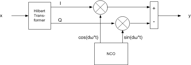
Figure 5. Frequency Shifter Implementation.
Now we’ll develop some Matlab code to shift the frequency of an input signal centered at 12 Hz by +3 Hz. First, we modify the Hilbert transformer used previously by replacing the Hamming window with a Blackman window. Compared to the Hamming window, this gives a more accurate passband response, at the expense of response flatness at low frequency. We will also quantize the coefficients to 12 bits.
    % 31-tap Hilbert transformer
    b= 2/pi * [-1/15 0 -1/13 0 -1/11 0 -1/9 0 -1/7 0 -1/5 0 -1/3 0 -1 0 1 0 …
               1/3 0 1/5 0 1/7 0 1/9 0 1/11 0 1/13 0 1/15];
    b1= b.*blackman(31)';                         % window the coefficients
    b1= round(b1*2^12)/2^12;                      % quantize coefficients
    b2= [0 0 0 0  0 0 0 0  0 0 0 0  0 0 0 1];     % delay of 15 (center tap of HT)
Now we’ll generate the input signal x and apply it to the Hilbert transformer. Rather than using a sinusoid, we’ll use a modulated pulse with approximately rectangular spectrum. The Matlab function to generate the pulse is listed in the Appendix.
fs= 100;                       % Hz sample frequency
Ts= 1/fs;
N= 2048;
n= 0:N-1;
fc= 12;                        % Hz carrier frequency
bw= 2;                         % Hz -3 dB bandwidth of modulated pulse
x= .5*modpulse(fc,bw,N,fs);    % modulated pulse with approx rect spectrum
% Apply modulated pulse to Hilbert transformer
I= filter(b2,1,x);             % I= center tap of HT filter
Q= filter(b1,1,x);             % Q= output of HT filter
Next we generate the NCO output and use it to shift the frequency. The modulus function is used to make the NCO’s phase accumulator roll-over when its value exceeds 1.
    df= 3;                              % Hz desired frequency shift
    u= mod(df*n*Ts,1);                  % phase accumulator
    theta= 2*pi*u;                      % phase
    y= I.*cos(theta) –Q.*sin(theta);    % final output
At this point, we can find the spectrum of the real output y. However, it’s instructive to look at the spectra of all of the signals in Figure 5. We have the real signals x and y, plus three complex quantities: the Hilbert transformer output; the NCO output; and the complex product of the NCO and Hilbert outputs. The complex quantities are easily calculated as follows:
    xc= I + j*Q;            % complex Hilbert transformer output
    nco= exp(j*theta);      % complex nco output
    yc= xc.*nco;            % complex product
We compute the spectrum of each quantity as follows:
    X= fft(x,N);          XdB= 20*log10(abs(x));
    XC= fft(xc,N);        XCdB= 20*log10(abs(XC));
    YC= fft(yc,N);        YCdB= 20*log10(abs(YC));
    NCO= psd(nco,N,fs);   NCOdB= 10*log10(abs(NCO));
    Y= fft(y,N);          YdB= 20*log10(abs(Y));
These spectra are shown in Figure 6, where we have shifted the portion of the spectrum above fs/2 to the range –fs/2 to 0. Figure 6a shows the spectrum of real input signal x, and Figure 6b shows that of the complex Hilbert output xc, which approximates an analytic signal. That is, it has negligible frequency components for f < 0. Figure 6c shows the spectrum of NCO signal exp(jθ), which is also analytic, having a single component at +3 Hz. Figure 6d shows the spectrum of the complex product. As you can see, the complex multiplication has shifted the center of xc from 12 Hz to 15 Hz. Finally, Figure 6e shows the spectrum of the real output y, centered at 15 Hz.
Had we multiplied two real signals instead of complex signals, we would have gotten duplicate spectra centered at 9 and 15 Hz: not a useful result. This shows the power of using complex signals. Finally, note that we didn’t need to know the frequency of the input signal – the frequency shifter works on any signal in the Hilbert transformer’s passband.
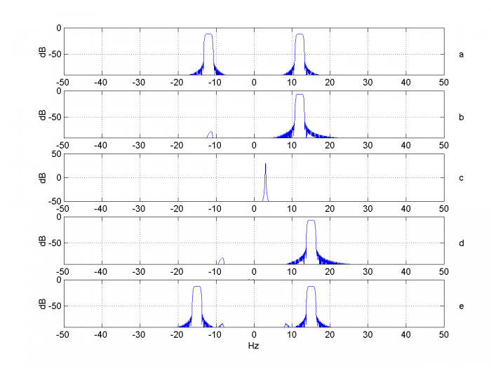
Figure 6. Spectra of signals within the frequency shifter.
a. real input X b. Hilbert output XC c. NCO output, df= 3 Hz
d. complex product YC e. Final output Y
Now let’s examine the purity of the output spectrum. The spectra of the real input signal x and real output signal y are plotted in Figure 7. The sideband at 9 Hz is caused by the Hilbert Transformer not having perfect response magnitude of 1. This is due to the truncation of coefficients to 31 taps and quantization of the coefficients.
While we’re looking at imperfections, we can also quantize the NCO phase and NCO output (LUT quantization). The following code quantizes these to 10 bits. The resulting output spectrum is shown in Figure 8.
    u= mod(df*n*Ts,1);                        % phase accumulator
    u= round(u*2^10)/2^10;                    % phase quantization
    theta= 2*pi*u;                            % quantized phase
    costheta= round(2^10*cos(theta))/2^10;    % NCO output quantization
    sintheta= round(2^10*sin(theta))/2^10;
    y= I.*costheta -Q.*sintheta;
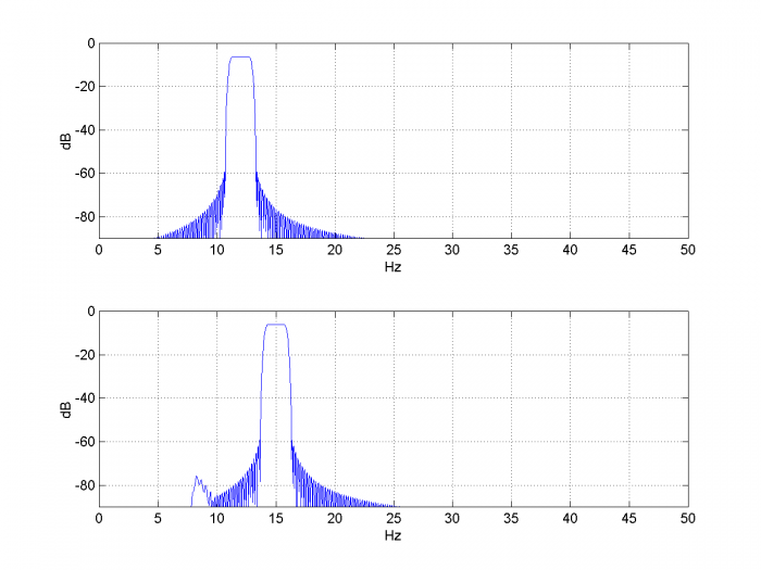
Figure 7.Spectra of frequency shifter input and output for fc= 12 Hz, df= 3 Hz,
HT length= 31 taps, HT quantization= 12 bits, fs= 100 Hz.
[h,f]= freqz(y,1,N,fs); H= 20*log10(abs(h));
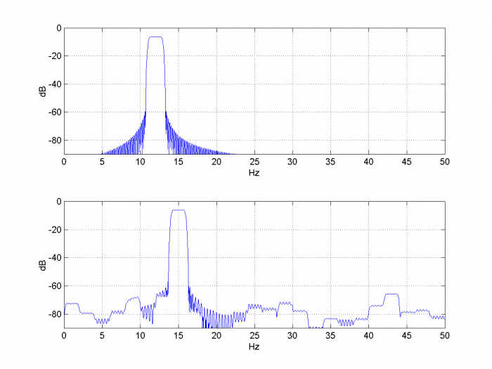
Figure 8.Spectra of frequency shifter input and output for fc= 12 Hz, df= 3 Hz,
HT length= 31 taps, HT quantization= 12 bits, fs= 100 Hz,
NCO phase quantization = 10bits, NCO LUT quantization= 10 bits.
Hilbert Transformer
Here we’ll touch on the math behind the Hilbert transformer, and we’ll look at basics of how to implement one. A more detailed description of the theory of the Hilbert transformer is presented in references [1,2].
An ideal discrete Hilbert transformer Q-channel output has frequency response:
$$H(z)= -j, \qquad 0\lt f \lt f_s/2$$
$$\qquad \qquad \qquad= j,\qquad -f_s/2 \lt f \lt 0 \qquad (2) $$
This response can only be approximated by a practical filter (skip ahead to Figure 11 for an example). The impulse response over -∞ < n < ∞ is:
$$h[n]=\frac{2}{\pi n},\qquad for\, n\, odd$$
$$\qquad \qquad \quad = 0,\qquad for\, n\, even \qquad (3)$$
This impulse response is non-causal, but it can be approximated by truncating, letting n =
–N/2 : N/2-1, where N is even and N+1 is the number of taps. The taps can then be multiplied by a window function. A block diagram of a 7-tap Hilbert Transformer is shown in Figure 9 [3], where the top diagram numbers the taps according to Equation 3, and the bottom diagram renumbers them to start with b0. The I-channel is taken as the center tap of the delay network, which corresponds to t = 0 in the ideal Hilbert transformer.
The Q-channel response of–j = e-jπ/2 gives a π/2 phase lag for a sinusoidal input. Thus, for I = cos(ωt), Q is sin(ωt). We can then define the complex signal I + jQ = cos(ωt) +jsin(ωt) = ejωt. Unlike the real input signal, this signal has no spectral component at -ω. Signals with no spectral components for f < 0 are called analytic signals.
In general, the output of the Hilbert transformer is analytic for input signals in its passband . For example, in the preceding section, the modulated pulse signal was transformed into an (approximately) analytic signal, with spectrum shown in Figure 6b.
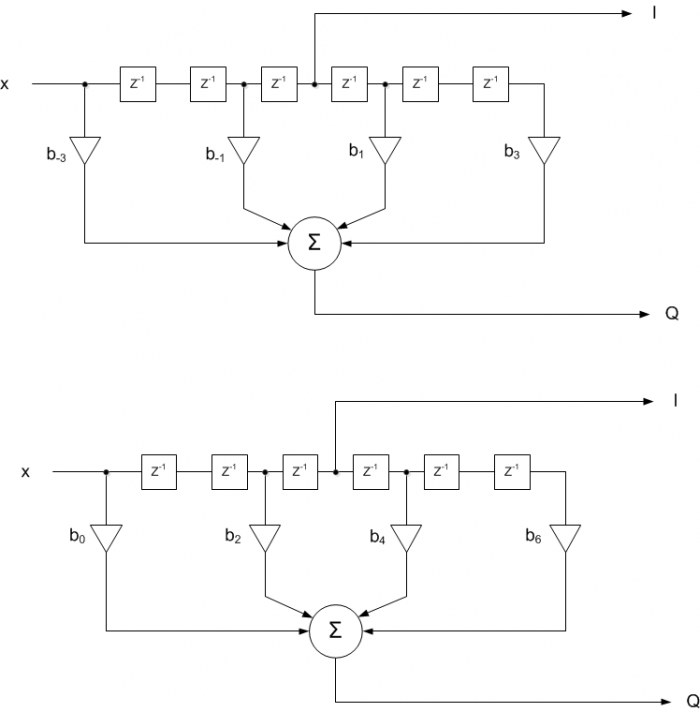
Figure 9. 7-tap Hilbert Transformer. Top: with taps numbered per Equation 3.
Bottom: with taps re-numbered to start with b0.
In the previous section, we implemented a 31-tap Hilbert transformer by windowing the truncated coefficients of Equation 3 with a Blackman window. Here is the code again:
     % 31-tap Hilbert transformer
    b= 2/pi * [-1/15 0 -1/13 0 -1/11 0 -1/9 0 -1/7 0 -1/5 0 -1/3 0 -1 0 1 0 …
               1/3 0 1/5 0 1/7 0 1/9 0 1/11 0 1/13 0 1/15];
    b1= b.*blackman(31)';                         % window the coefficients
    b1= round(b1*2^12)/2^12;                      % quantize coefficients
    b2= [0 0 0 0  0 0 0 0  0 0 0 0  0 0 0 1];     % delay of 15 (center tap of HT)
These coefficients are plotted in Figure 10. Now let’s compute frequency response. In making a realizable filter, we delayed the input by 15 samples to create the I channel. Thus we need to calculate the response with respect to this delayed version of the input. The Matlab code is listed below and the response is plotted in Figure 11. As you can see, the response is pure imaginary and deviates from Equation 2 at low frequencies and near fs/2. When using the Hilbert transformer, we need to make sure that the signal frequency is in the flat part of the response.
    N= 1024;
    k= -N/2:N/2-1;
    f= k*fs/N;
    h_Q= fft(b1,N);            % h_Q = response of b1
    h_I= fft(b2,N);            % h_I = response at center tap (delay of 15 samples)
    h= h_Q./h_I;
    h= fftshift(h);            %shift dc to center (swap left and right halves of h)
    plot(f,imag(h))
Finally, regarding this window method of Hilbert transformer design: while straightforward, it is typically not the most efficient method. An efficient approach uses the Parks-McClellan equiripple FIR design algorithm, which is implemented by the Matlab function firpm [4]. This function has a mode specifically for Hilbert transformer design.
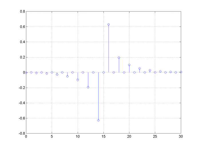
Figure 10. Coefficients of 31-tap Hilbert Transformer.
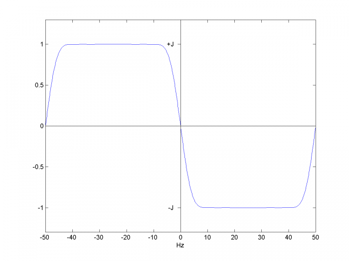
Figure 11. Frequency Response of 31-tap Hilbert transformer, fs= 100 Hz
(Blackman window)
References
1. Mitra, Sanjit K., Digital Signal Processing, 2nd Ed., McGraw-Hill, 2001, section 11.7.
2. Lyons, Richard G., Understanding Digital Signal Processing, 2nd Ed., Pearson, 2004, Ch. 9.
3. Lyons, p 374.
4. Mathworks website, https://www.mathworks.com/help/signal/ref/firpm.html
March, 2018 Neil Robertson
Appendix Matlab Function to Generate a Modulated Pulse
This function generates a modulated pulse having an approximately rectangular spectrum. The pulse envelope response is generated using a window-based FIR lowpass filter. An example pulse output is shown in Figure A.1, and its spectrum is shown in Figure A.2.
%function y = modpulse(fc,bw,N,fs)  3/10/18 Neil Robertson
%
% Modulated pulse with approximately rectangular spectrum
% fc = carrier freq, Hz
% bw = -3 dB bw of modulated pulse spectrum, Hz
% N = pulse length including padding, samples.N must be a multiple of 8.
% fs = sample frequency, Hz
%
% example:y= modpulse(20,4,1024,100)
%
function y = modpulse(fc,bw,N,fs)
if mod(N,8)~=0
    error('N must be a multiple of 8')
end
M= N/4;                        % FIR filter number of taps
Ts= 1/fs;
n= 0:N-1;
f1= bw/2;
win= kaiser(M,5);
b= fir1(M-1,2*f1/fs,win);        % window-based FIR coeffs, M taps
pad= zeros(1,(N-M)/2);
d= [pad b pad];                  % padded pulse with total length = N
x= cos(2*pi*fc*n*Ts);            % carrier
y= x.*d;                         % modulated pulse
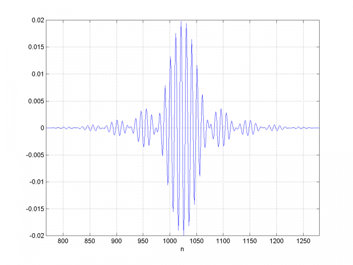
Figure A.1 512 samples of modulated pulse y= modpulse(fc,bw,N,fs)
fc= 10, bw= 2, N= 2048, fs= 100.
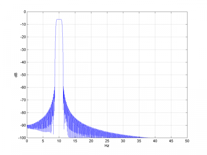
Figure A.2 Spectrum of modulated pulse.
- Comments
- Write a Comment Select to add a comment

The spectrum in the bottom panel of your Figure 8 is, to quote Mr. Spock, "fascinating." I'll have to copy your code and experiment with various levels of quantization. (Thanks for including your MATLAB code in this blog.)

Rick,
Yes, I have not looked closely at the effects of quantizing the NCO phase and LUT. I'll be interested to hear any insights you have.
Note that the PDF file has an appendix B that contains the frequency shifter code (but does not include the five lines of code that perform the NCO quantization).
regards,
Neil
Can you unpack why you subtract Q from I in the equation:
y= I.*costheta -Q.*sintheta;
to obtain the real result y?
Hi,
The formula for this is Equation 1 near the beginning of the post:
y=Re{(I+jQ)ejθ}y=Re{(I+jQ)ejθ}
=Re{(I+jQ)(cosθ+jsinθ}=Re{(I+jQ)(cosθ+jsinθ}
y=Icosθ−Qsinθ (1)
The minus sign arises because
jQ* jsin(theta) = j*j*Q*sin(theta) = -Qsin(theta)
regards,
Neil
Thanks for the quick response!
Hi Neil.
Can you unpack how you knew what the word "unpack" meant?
(Perhaps mpettigr1 works in the Marketing Dept. of some company. Marketers love to create confusing new meanings for everyday words.)
Rick,
I think this is one of those words that journalists use. As in "Can you unpack what he means by Democratic Socialism?"
I can't recall when I first started hearing it, probably in the last decade or so ... or two decades or three.
Hi Rick,
This is mpettigr1. I'm neither a marketer nor a journalist, but an engineer for 25+ years. Never thought of the word 'unpack' as controversial. :-)
From Merriam-Webster definition, 3rd entry, "to analyze the nature of by examining in detail : explicate unpack a concept"
https://www.merriam-webster.com/dictionary/unpack
While I'm here, Neil, thanks for the great article. It cleared up a few things I hadn't thought of in a while.
Rick, well, thanks for everything. I've read many of your articles and books. You're a great teacher!
I'm trying to replicate frequency shift algorithm in OpenWire Studio by draging DSP components from palette. It look like I don't understood exacly how it works and need some help from specialist.
Above diagram show how I start. Is it good start? I haven't idea how to finish. I will be appriciated for help (this task is to complicated to me as start with DSP). Based on this model I would like to prepare program in C++ Rad Studio.
Hi Superviper,
Sorry, I'm not familiar with OpenWire Studio. I'm guessing it would be easier (and safer) to manually convert the Matlab code in my post to C++.
regards,
Neil
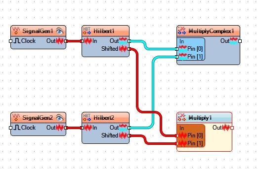
Let's consider that SignalGen1(500Hz) is the signal which I would like to shift and SignalGen2(100Hz) is the shifting signal.
I would like shift SignalGen1 by 100Hz.
I'm looking for methodology. I try to do Hilbert for SignalGen1 and SignalGen2. Then I multiplay Complex path of SignalGen1 by Complex path SignalGen2. I have done the same for real path. Am I'm right doing like that?
Superviper,
I think your terminology is a little confused. There is a real path and an imaginary path (not real and complex). I call the real path "I" (for in-phase) and the imaginary path "Q" (for quadrature-phase).
You need two real multipliers (no complex multiplier is used) and a summer, as shown in Figure 5 of the post. Also, it would be simpler to use an NCO with sine and cosine outputs instead of the real source SignalGen2 -- then you would only need one Hilbert Transformer.
regards,
Neil
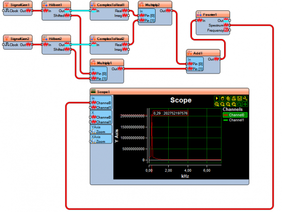
Dear Neil - your inspiration help me to finish and simulate block diagram in OpenWire Studio. It's software which help to simulate working Delphi/C++ components in easy form by draging DSP components and wire connections.
Below is what I did base on your suggestions and work perfectly. SignalGen1 is 500Hz and SignalGen2 is 200Hz and on scope you can see result which i 300Hz (Marker show 0,29kHz Peak). Simulation show that block diagram is ok so now time for programming ;)
Superviper,
Great! One thing to be on the look-out for: The Hilbert transformer response should be flat at the input frequency. For example, in Figure 11, it is flat from 10 to 40 Hz (linear amplitude scale).
regards,
Neil
I was to early happy. SignalGen1 is 500Hz and SignalGen2 is 200Hz (both sinusoid). When I do FFT and plot it on scope it's look like SignalGen1 is shifted 200Hz - so I was happy to achieve it - but when I listen output it sound like pink noise.
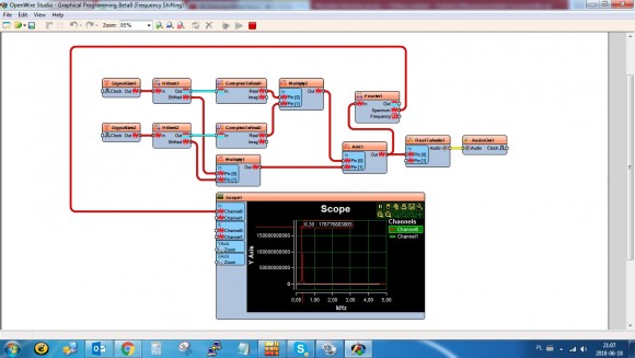
When I have done oscilogram it look like below

I have solved the issue :) SignalGen1 and SignalGen2 amplitude was high. When SignalGen1 is multipy by SignalGen2 amplitude is multiply what make output override. This was the problem that insteed nice sound of sinusoid I heard something similar to pink noise. Thank you all for support :)
Excellent! I guess you meant to say "output overflow" and not "output override".
Neil
Yes correct

Hi Neil,
Three years on, and I'm finding your article very interesting and informative.
For those interested in the Hilbert transform, I also found this Iowa Hills webpage useful - there is a free standalone application which can be downloaded and used for Hilbert design.
Best Regards,
Woodpecker
Thanks Woodpecker. Looks like we should give Iowa a try.
Neil
To post reply to a comment, click on the 'reply' button attached to each comment. To post a new comment (not a reply to a comment) check out the 'Write a Comment' tab at the top of the comments.
Please login (on the right) if you already have an account on this platform.
Otherwise, please use this form to register (free) an join one of the largest online community for Electrical/Embedded/DSP/FPGA/ML engineers:


