


Use Matlab Function pwelch to Find Power Spectral Density – or Do It Yourself
In my last post, we saw that finding the spectrum of a signal requires several steps beyond computing the discrete Fourier transform (DFT)[1]. These include windowing the signal, taking the magnitude-squared of the DFT, and computing the vector of frequencies. The Matlab function pwelch [2] performs all these steps, and it also has the option to use DFT averaging to compute the so-called Welch power spectral density estimate [3,4].
In this article, I’ll present some examples to show how to use pwelch. You can also “do it yourself”, i.e. compute spectra using the Matlab fft or other fft function. As examples, the appendix provides two demonstration mfiles; one computes the spectrum without DFT averaging, and the other computes the spectrum with DFT averaging. (Note: I have also created a simplified Matlab PSD function based on pwelch: see this post.)
We’ll use this form of the function call for pwelch:
[pxx,f]= pwelch(x,window,noverlap,nfft,fs)
The input arguments are:
x input signal vector
window window vector of length nfft
noverlap number of overlapped samples (used for DFT averaging)
nfft number of points in DFT
fs sample rate in Hz
For this article, we’ll assume x is real. Let length(x) = N. If DFT averaging is not desired, you set nfft equal to N and pwelch takes a single DFT of the windowed vector x. If DFT averaging is desired, you set nfft to a fraction of N and pwelch uses windowed segments of x of length nfft as inputs to the DFT. The |X(k)|2 of the multiple DFT’s are then averaged.
The output arguments are:
pxx power spectral density vector, W/Hz
f vector of frequency values from 0 to fs/2, Hz
The length of the output vectors is nfft/2 + 1 when nfft is even. For example, if nfft= 1024, pxx and f contain 513 samples. pxx has units of W/Hz when x has units of volts and load resistance is one ohm.
Examples
The following examples use a signal x consisting of a sine wave plus Gaussian noise. Here is the Matlab code to generate x, where sine frequency is 500 Hz and sample rate is 4000 Hz:
    fs= 4000;                % Hz sample rate
    Ts= 1/fs;
    f0= 500;                 % Hz sine frequency
    A= sqrt(2);              % V sine amplitude for P= 1 W into 1 ohm.
    N= 1024;                 % number of time samples
    n= 0:N-1;                % time index
    x= A*sin(2*pi*f0*n*Ts) + .1*randn(1,N);    % 1 W sinewave + noise
The power of the sine wave into a 1-ohm load is A2/2 = 1 watt. In the following, examples 1 and 2 compute a single DFT, while example 3 computes multiple DFT’s and averages them. Example 4 calculates C/N0 for the spectrum of Example 3.
We’ll start out with a rectangular window. Note the sinewave frequency of 500 Hz is at the center of a DFT bin to prevent spectral leakage [5]. Here is the code to compute the spectrum. Since we are not using DFT averaging, we set noverlap= 0:
    nfft= N;
    window= rectwin(nfft);
    [pxx,f]= pwelch(x,window,0,nfft,fs);    % W/Hz power spectral density
    PdB_Hz= 10*log10(pxx);                  % dBW/Hz
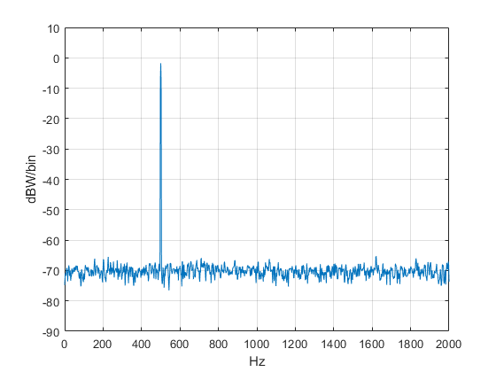
The resulting spectrum is plotted in Figure 1, which shows the component at 500 Hz with amplitude of roughly -6 dBW/Hz. How does this relate to the actual power of the sinewave for a 1-ohm load resistance? To compute the power of the spectral component at 500 Hz, we need to convert the amplitude in dBW/Hz to dBW/bin as follows. First, convert W/Hz to W/bin:
Pbin (W/bin) = pxx (W/Hz) * fs/nfft (Hz/bin) (1)
Then, we have in dB:
PdB_bin = 10*log10(pxx*fs/nfft) dBW/bin (2)
Or PdB_bin = PdB_Hz + 10*log10(fs/nfft) dBW/bin
If we set the noise amplitude to zero, we get PdB_Hz = -5.9176 dB/Hz and
PdB_bin= -5.9176 dBW/Hz + 10log10(4000/1024) = 0 dBW = 1 watt
So we are reassured that the amplitude of the spectrum is correct. This motivates us to try the next example, which displays the spectrum in dBW/bin.
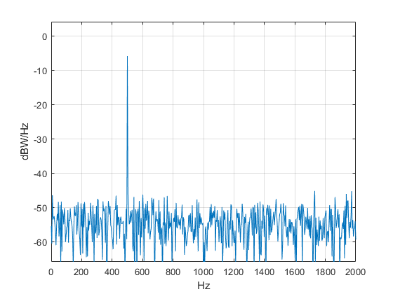
Figure 1. Spectrum in dBW/Hz
To find the spectrum in dBW/bin, the code is the same as Example 1, except we use Equation 2 to find PdB_bin:
    nfft= N;
    window= rectwin(nfft);
    [pxx,f]= pwelch(x,window,0,nfft,fs);      % W/Hz power spectral density
    PdB_bin= 10*log10(pxx*fs/nfft);           % dBW/bin
The spectrum is shown in the top plot of Figure 2. As expected, the component at 500 Hz has power of 0 dBW. Note that the amplitude of a sine’s spectral component in dBW/bin is constant vs nfft, while the amplitude in dBW/Hz varies vs. nfft. If we now replace the rectangular window with a hanning window:
window= hanning(nfft);
We get the spectrum in the bottom plot of Figure 2. The peak power is now less than 0 dBW, because the power is spread over several frequency samples of the window. Nevertheless, this is a more useful window than the rectangular window, which has bad spectral leakage when f0 is not at the center of a bin.
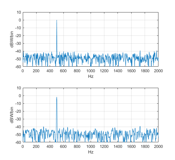
Figure 2. Spectra in dBW/bin Top: rectangular window
Bottom: hanning window
Example 3. DFT averagingFor this example, fs, Ts, f0, A, and nfft are the same as for the previous examples, but we use N= 8*nfft time samples of x. pwelch takes the DFT of Navg = 15 overlapping segments of x, each of length nfft, then averages the |X(k)|2 of the DFT’s. The segments of x are shown in Figure 3, where we have set the number of overlapping samples to nfft/2 = 512.
In general, if there are an integer number of segments that cover all samples of N, we have [4]:
(Navg – 1)*D + nfft = N (3)
Where D = nfft – noverlap. For our case, with D = nfft/2 and N/nfft = 8, we have
Navg = 2*N/nfft -1 = 15.
For a given number of time samples N, using overlapping segments lets us increase Navg compared with no overlapping. In this case, overlapping of 50% increases Navg from 8 to 15. Here is the Matlab code to compute the spectrum:
    nfft= 1024;
    N= nfft*8;                                % number of samples in signal
    n= 0:N-1;
    x= A*sin(2*pi*f0*n*Ts) + .1*randn(1,N);   % 1 W sinewave + noise
    noverlap= nfft/2;                         % number of overlapping time samples
    window= hanning(nfft);
    [pxx,f]= pwelch(x,window,noverlap,nfft,fs);  % W/Hz  PSD
    PdB_bin= 10*log10(pxx*fs/nfft);              % dBW/bin
The resulting spectrum is shown in Figure 4. Compared to the no-averaging case in Figure 2, there is less variation in the noise floor. DFT averaging reduces the variance σ2 of the noise spectrum by a factor of Navg, as long as noverlap is not greater than nfft/2 [6].
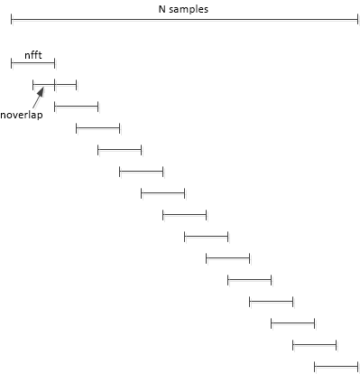
Figure 3. Overlapping segments of signal x for N = 8*nfft and noverlap = nfft/2 (50%).
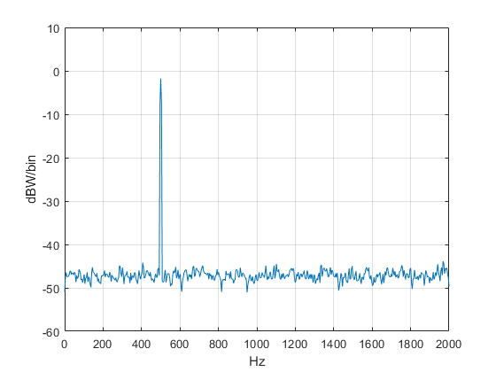
Figure 4. Spectrum with Navg = 15 and noverlap= nfft/2= 512.
Reducing the noise variance by DFT averaging makes calculation of the noise level and thus carrier-to-noise ratio (C/N) more accurate. Let’s calculate C/N0 for the signal of Example 3, where N0 is the noise power in a 1 Hz bandwidth.
First, we’ll find the power of the sinewave (the “C” in C/N0) by performing a peak search on the dBW/bin spectrum, then adding the spectral components near the peak to get the total power. This is necessary because windowing has spread the power over several frequency samples.
    y= max(PdB_bin);                 % peak of spectrum
    k_peak= find(PdB_bin==y);        % index of peak
    Psum= fs/nfft * sum(pxx(k_peak-2:k_peak+2));    % W sum power of 5 samples
    C= 10*log10(Psum)                % dBW carrier power
The peak power of 0 dBW is shown by the marker in the left plot of Figure 4. Now we’ll find N0 from the dBW/Hz spectrum. Choosing f = 800 Hz, we have:
    PdB_Hz= 10*log10(pxx);       % dBW/Hz
    f1= 800;                     % Hz
    k1= round(f1/fs *nfft);      % index of f1
    No= PdB_Hz(k1)               % dBW/Hz Noise density at f1
The N0 marker is shown in the right plot of Figure 4. Figure 5 combines the dBW/bin and dBW/Hz plots in one graph. C/N0 is just:
CtoNo= C - No; % dB (1 Hz)
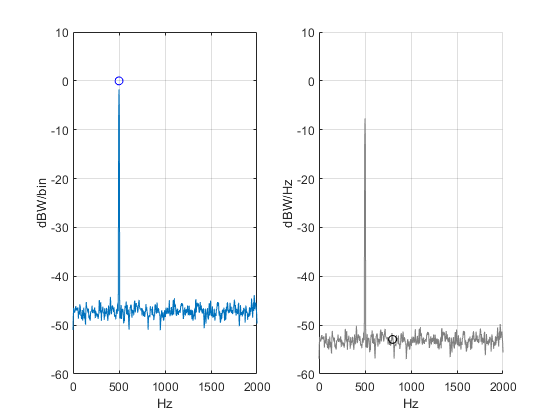
Figure 5. Left: Spectrum in dBW/bin with marker showing the power of the sinewave.
Right: Spectrum in dBW/Hz with marker at 800 Hz showing N0.
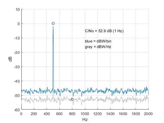
Figure 6. Spectrum in dBW/bin (blue) and dBW/Hz (grey).
Appendix Matlab Code to compute spectra without using pwelch
These examples use the Malab fft function to compute spectra. See my earlier post [7] for derivations of the formulas for power/bin and normalized window function.
Demonstrate Spectrum Computation/ No Averaging
%spectrum_demo.m   1/3/19  Neil Robertson
% Use FFT to find spectrum of sine + noise in units of dBW/bin and dBW/Hz.
fs= 4000;                        % Hz sample frequency
Ts= 1/fs;
f0= 500;                         % Hz sine frequency
A= sqrt(2                        % V sine amplitude for P= 1 W into 1 ohm.
N= 1024;                         % number of time samples
nfft= N;                         % number of frequency samples
n= 0:N-1;                        % time index
%
x= A*sin(2*pi*f0*n*Ts) + .1*randn(1,N);    % 1 W sinewave + noise
w= hanning(N);                   % window function
window= w.*sqrt(N/sum(w.^2));    % normalize window for P= 1
xw= x.*window';                  % apply window to x
%
X= fft(xw,nfft);                 % DFT
X= X(1:nfft/2);                  % retain samples from 0 to fs/2
magsq= real(X).^2 + imag(X).^2;  % DFT magnitude squared
P_bin= 2/nfft.^2 * magsq;        % W/bin power spectrum into 1 ohm
P_Hz= P_bin*nfft/fs;             % W/Hz power spectrum
%
PdB_bin= 10*log10(P_bin);        % dBW/bin
PdB_Hz= 10*log10(P_Hz);          % dBW/Hz
%
k= 0:nfft/2-1;                   % frequency index
f= k*fs/nfft;                    % Hz frequency vector
%
%
plot(f,PdB_bin),grid
axis([0 fs/2 -60 10])
xlabel('Hz'),ylabel('dBW/bin')
title('Spectrum with amplitude units of dBW/bin')
figure
y= max(PdB_Hz);
plot(f,PdB_Hz),grid
axis([0 fs/2 y-60 y+10])
xlabel('Hz'),ylabel('dBW/Hz')
title('Spectrum with amplitude units of dBW/Hz')
Demonstrate Spectrum Computation with Averaging
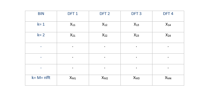
Suppose we have segmented a signal x into four segments of length nfft, that could be overlapped. If we window each segment and take its DFT, we have four DFT’s as shown in Table A.1. Here, we have defined M= nfft and we have numbered the FFT bins from 1 to M (instead of 0 to M - 1).
Table A.1 DFT’s of four segments of the signal x.
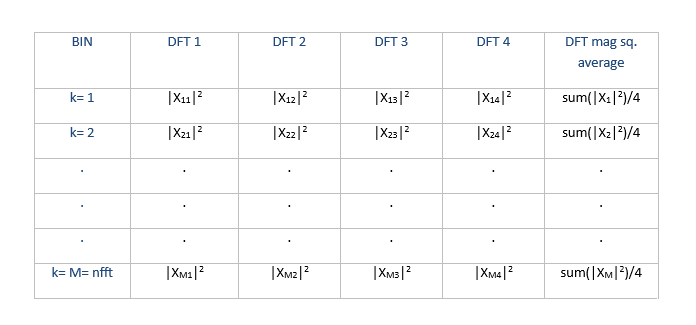
Now we form the magnitude-squared of each bin of the four DFT’s, as shown in Table A.2 If we then sum the magnitude-square values of each bin over the four DFT’s and divide by 4, we obtain the average magnitude-squared value, as shown in the right column. Finally, we scale the magnitude-squared value to obtain the averaged power per bin [7] or averaged power per Hz:
Pbin(k) = 2/M2 * sum(|Xk|2)/4 W/bin (A.1)
PHz(k)= Pbin(k)*M/fs W/Hz (A.2)
Or
PHz(k)= 2/(M*fs) * sum(|Xk|2)/4 W/Hz (A.3)
PHz(k) is the Welch power spectral density estimate.
Table A.2 Magnitude-square values of Four DFT’s, and their average (right column).
The following example m-file uses Navg = 8, summing 8 values of each |X(k)|2 and dividing by 8. For simplicity, noverlap = 0 samples. Another option for averaging, useful for the case where DFT’s are taken continuously, is exponential averaging, which basically runs the |X(k)|2 through a first-order IIR filter [8].
%spectrum_demo_avg  1/3/19 Neil Robertson
% Perform DFT averaging on signal = sine + noise
% noverlap = 0
% Given signal x(1:8192),
%
%            |x(1)    x(1025) . . . . x(7169)|
%            |x(2)    x(1026) . . . . x(7170)|
% xMatrix=   | .         .               .   |
%            | .         .               .   |
%            |x(1024) x(2048) . . . . x(8192)|
%
%
fs= 4000;                        % Hz sample frequency
Ts= 1/fs;
f0= 500;                         % Hz sine frequency
A= sqrt(2                        % V sine amplitude for P= 1 W into 1 ohm
nfft= 1024;                      % number of frequency samples
Navg= 8;                         % number of DFT's to be averaged
N= nfft*Navg;                    % number of time samples
n= 0:N-1;                        % time index
x= A*sin(2*pi*f0*n*Ts) + .1*randn(1,N);    % 1 W sinewave + noise
w= hanning(nfft);                          % window function
window= w.*sqrt(nfft/sum(w.^2));           % normalize window for P= 1 W
%
% Create matrix xMatrix with Navg columns,
% each column a segment of x of length nfft
xMatrix= reshape(x,nfft,Navg);
magsq_sum= zeros(nfft/2);
for i= 1:Navg
    x_column= xMatrix(:,i);
    xw= x_column.*window;                % apply window of length nfft
    X= fft(xw);                          % DFT
    X= X(1:nfft/2);                      % retain samples from 0 to fs/2
    magsq= real(X).^2 + imag(X).^2;      % DFT magnitude squared
    magsq_sum= magsq_sum + magsq;        % sum of DFT mag squared
end
mag_sq_avg= magsq_sum/Navg;              % average of DFT mag squared
P_bin= 2/nfft.^2 *mag_sq_avg;            % W/bin power spectrum
P_Hz= P_bin*nfft/fs;                     % W/Hz power spectrum
PdB_bin= 10*log10(P_bin);                % dBW/bin
PdB_Hz= 10*log10(P_Hz);                  % dBW/Hz
k= 0:nfft/2 -1;                          % frequency index
f= k*fs/nfft;                            % Hz frequency vector
%
plot(f,PdB_bin),grid
axis([0 fs/2 -60 10])
xlabel('Hz'),ylabel('dBW/bin')
title('Averaged Spectrum with amplitude units of dBW/bin')
figure
plot(f,PdB_Hz),grid
axis([0 fs/2 -60 10])
xlabel('Hz'),ylabel('dBW/Hz')
title('Averaged Spectrum with amplitude units of dBW/Hz')
References
- Robertson, Neil, “Evaluate Window Functions for the Discrete Fourier Transform” https://www.dsprelated.com/showarticle/1211.php
- Mathworks website https://www.mathworks.com/help/signal/ref/pwelch.html
- Oppenheim, Alan V. and Shafer, Ronald W., Discrete-Time Signal Processing, Prentice Hall, 1989, pp. 737—742.
- Welch, Peter D., “The Use of Fast Fourier Transform for the Estimation of Power Spectra: A Method Based on Time Averaging Over Short, Modified Periodograms”, IEEE Trans. Audio and Electroacoustics, vol AU-15, pp. 70 – 73, June 1967. https://www.utd.edu/~cpb021000/EE%204361/Great%20DSP%20Papers/Welchs%20Periodogram.pdf
- Lyons, Richard G., Understanding Digital Signal Processing, 2nd Ed., Prentice Hall, 2004, section 3.8.
- Oppenheim and Shafer, p. 738.
- Robertson, Neil, “The Power Spectrum”, https://www.dsprelated.com/showarticle/1004.php
- Lyons, section 11.5.
Neil Robertson January, 2019


- Comments
- Write a Comment Select to add a comment
Hi Neil
thank you very much,
there is something that has been confusing me, I hope I can find an answer please.
I have noticed that as we change nfft, the power spectral density in dB/bin is always constant, but the PSD in dB/Hz would change. which means that I am getting different PSD (dB/Hz) result as I change nfft.
is that normal in theory? what is the reason behind this?
thanks

AmroGonem,
Indeed, the PSD in W/bin or dB/bin is constant vs. nfft. You can find the formula for PSD in Watts/bin in an earlier post I wrote.
To find PSD in W/Hz given PSD in W/bin, use this formula:
PSD (W/Hz) = PSD (W/bin)*nfft/fs (1)
nfft/fs has units of bins/Hz.
So given that the power in W/bin is constant vs nfft, equation 1 tells us that the power in W/Hz is proportional to nfft.
I find computing power in W/bin or dB/bin is usually more clear. Also, you can read the power of a sine wave directly from a plot (although there is some processing loss due to the window function). Note that swept spectrum analyzers' displays are essentially equivalent to dB/bin, except when in marker-noise mode.
regards,
Neil
Thank you very much
Thanks Neil for the very informative article. I'm just wondering at the end where you calculate the SNR, should you have taken the processing gain into account. The noise floor as shown in figure 6 is lowered by the processing gain?
Hi gartlant,
In figure 6, the left plot has amplitude units of dBW/bin, and the right plot has amplitude units of dBW/Hz. This is the reason for the difference in noise floor (and difference in carrier level as well).
Regarding processing gain due to DFT averaging: If you look at the un-averaged spectrum in Figure 2, and you try to put a marker on the noise, you can get a 20 dB variation of the noise reading depending on exactly where you place the marker. In the averaged spectrum of figure 5 and 6, we have less variation in the noise floor, so maybe only 6 dB variation. You can say processing gain is inherent in the plotted spectrum.
regards,
Neil
Hi Neil, thank you for the brilliant article. I am new to DSP and Matlab and will be using both to analyse long term acoustic data. Can you explain/point me to any resources for why I would/wouldn't use DFT averaging? I want to apply pwelch using a Hanning window with 50% overlap, in 1Hz frequency bins and ultimately transform the results (using 10log10?) to get values in db re 1 micro Pascal. How does this impact the nfft if my sampling rate is 144kHz? Do the two even relate? Thanks for any help you can offer,
Hi,
What is the maximum frequency of interest of your signal?
regards,
Neil
Thank you for sharing knowledge in DSP, it is very helpful. I'm learning a lot, by I still need your help.
I'm using a GNSS receiver for some measurements and some times the results are
not what I inspected. Researches in the Internet tell me that by plotting the power spetrum (density) of the signal I can see if there are some interferences or any others signals that can disturb the receiver.
For GNSS receivers, a Interference threshold mask is defined by ICAO in the GNSS SARPs (Section 3.7 of appendix B of
ICAO Annex 10 to the Chicago Convention, amendment 76, Nov. 2001), and helps to identify interferences, or others unwanted signals.
To fullfill this requirements I assume that I need to plot the power spectrum density from noise floor of the signal that is approx. -164.5 dBW.
Data:
I/Q samples
Number of Samples 2000
Sampling frequency 60 MHz
Frequency(Center) 1584 MHz
My questions:
1) Is my thinking correct?
2) can I plot this power spectrum density with I/Q Samples?
3) How or references?
If more data are needed, please let me know, I will try provide these data.
Thank you against for your help.
Hi,
You can look at the spectrum of the I or Q channel using pwelch. You should use 2^N samples, for example 2048. With 2048 samples, the frequency resolution is 60E6/2048 = 29.3 kHz.
The receiver converts the signal centered at 1584 MHz to baseband I/Q. The baseband frequency range is 0 to fs/2 = 0 to 30 MHz.
You can also find the spectrum of the complex baseband signal I + jQ, although I did not discuss that in the post.
regards,
Neil
Hi Neil,
Dank you.
I was not clear enough.
What are the steps to estimate self noise (noise floor), if there is one?
Best regards
Levi
Levi,
There is not a short answer to your question. Here are a couple of references that may apply:
https://literature.cdn.keysight.com/litweb/pdf/5952-8255E.pdf
regards,
Neil
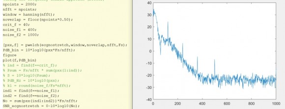
Hi, thanks for the great article. I'm trying to calculate the SNR of my ECG signal. But I do not have a characteristic peak that I'm looking for. Instead, I'm using a frequency range (everything less than 40 Hz) and summing over that frequency range, just as you did with the additional 5 samples around your peak. My sampling rate is 2000.
I'm having an issue in determining how I should calculate the noise. I thought that I should use a range of of frequencies from the dB/Hz spectrum, instead of choosing a single point, as you showed. But when I do use that range of frequencies (800-900 Hz), the SNR values are unrealistically high. However, if I use the same range from the dB/bin spectrum (which is not what you mentioned in the article), then the SNR value is reasonable. Below is my code:
npoints = 2000;
nfft = npoints;
window = hanning(nfft);
noverlap = floor(npoints*0.50);
crit_f = 40;
noise_f1 = 800;
noise_f2 = 900;
[pxx,f] = pwelch(ecgnostretch,window,noverlap,nfft,Fs);
PdB_bin = 10*log10(pxx*Fs/nfft);
figure
plot(f,PdB_bin)
ind = find(f==crit_f);
Psum = Fs/nfft * sum(pxx(1:ind));
S = 10*log10(Psum);
PdB_Hz = 10*log10(pxx);
% k1 = round(noise_f/Fs*nfft);
ind1 = find(f==noise_f1);
ind2 = find(f==noise_f2);
No = Fs/nfft * mean(pxx(ind1:ind2)); %for noise, we should average, that's why use mean instead of sum
SNR_ecgnostretch = S-No;
Could you offer any suggestions as to if this is an accurate way to calculate the SNR?
Hi fazeem,
I think you have a mistake in computing No: it would need to be a dB quantity. I am not familiar with ECG; however, here is an example of SNR calculation. Note that SNR and S/No are two different things. Since you say you are interested in SNR, that's what I calculate here. The result is SNR_dB = 40.
regards,
Neil
%snr1.m 2/17/20 nr
% compute SNR of sine + gaussian noise
% generate signal
fs= 4000;
Ts= 1/fs;
f0= 500;
A= sqrt(2);
N= 8192;
n= 0:N-1;
% signal with SNR of 40 dB (20 log10(.01) = -40 dBW)
x= A*sin(2*pi*f0*n*Ts) + .01*randn(1,N);
nfft= 2048;
noverlap= nfft/2;
window= hanning(nfft);
[p,f]= pwelch(x,window,noverlap,nfft,fs);
dBW_bin= 10*log10(p*fs/nfft);
% sum noise, excluding carrier neighborhood
sump= sum(p(1:252)) + sum(p(262:end));
pnoise_bin= sump*fs/nfft; % total noise power in W
N= 10*log10(pnoise_bin); % dBW
SNR_dB= 0 - N % note: signal power is 0 dBW
plot(f,dBW_bin),grid
axis([0 fs/2 -90 10])
xlabel('Hz'),ylabel('dBW/bin')
Thank you very much for your reply. For ECG, I don't have any characteristic peak, so I'm just using the frequency range between 0-40 Hz as that is the relevant frequency range for this signal.
It seems that, for the noise, I need to select my entire noise range as that outside my frequency range of interest, i.e. everything above 40 Hz. If I do that, I still get a negative SNR, which is probably due to some of the noise values being above 0 dB. I think this is due to my data acquisition system as all my PSD plots show similar behavior. If I pick a frequency range which is for sure in the noise floor (i.e. 800 to 1000 Hz), I can get an SNR of about 1, which doesn't make sense just by looking at the raw signal.
Attached is an example of the PSD plot (dbW/bin on the y axis, frequency on x) I'm getting along with the code. Below that is a picture of one of the signals.

Also, why is 0 used as the power of the signal?
Fazeem,
The power of the signal in my example is 1 watt = 0 dBW.
Looking at your signal spectrum, I guess it makes sense to sum the power/bin from 0 to 40 Hz. One way to find the noise power would be to use a signal with the transducer not attached to a person (or attached to a dead person), then just sum the noise spectrum.
If that is not possible, you could assume that the noise floor is flat. Then you could find No near 800 Hz or so, where No = 10*log10(pxx) at a single point (note pxx is in W/Hz). You could average No over a few nearby points if desired. Then total noise would be No + 10*log10(fs/2) dBW.
Again, I don't know anything about ECG. I am not responsible for the use or misuse of this advice.
regards,
Neil
Thank you again for the response. I think what you've mentioned is definitely logical and applies to my case actually. I've reviewed some literature and this seems to be a plausible strategy. Thank you for the comments.
Hello ,
thank you for this article.
I would like to ask you what are the best way to calculate the parameters used in pwelch function.
I have a signal length of N= 5678000 and a sampling rate of fs= 1000.
Then I divide this signal in 3 depending on the onset and offset of a stimulus. For example N1= 1126535, N2=951465, N3=3600000.
I'm using the pwelch function in matlab but I don know what are the best parameters to choose for the window, the noverlap and the nfft.
I'm using now :
[pxx1,f1] = pwelch(BigMatPre(chs(e),:),2000,1000,2000,fs);
(BigMatPre is my signal)
All my best,
sarah
Sarah,
In my post, I use 5 inputs to pwelch, but you are showing 6 inputs, so I'm a little confused.
First of all, the computation will be faster if you choose nfft as a power of 2: you could use 2048 instead of 2000, although then the frequency step would not be a simple fraction.
Frequency resolution depends on nfft: For fs= 1000 and nfft = 2000, you have a resolution of fs/nfft = 0.5 Hz per bin. Higher values of nfft give better resolution at the expense of less spectrum averaging. So you may want to try different values of nfft to get a feeling for the trade-off. For example, you could try nfft = 4000 (or 4096).
The choice of noverlap = nfft/2 is probably OK.
For a window, you could start with a Hanning window. See my post discussing window functions:
https://www.dsprelated.com/showarticle/1211.php
regards,
Neil
Thank you for your answer
BigMatPre(chs(e),:) is because is a loop analysing the pwelch for e row.
I have an other question if you can help me.
I then want to compare the PSD of different groups, for example between the frequency range [40-80] but I m confuised. Is it good to compare the mean of a normalize PSD (mean of PSD value between 40-80 / mean of the PSD along [0.5-80] or the area under the curve?
Your article is really useful
thak you
Sorry, I don't understand the question.
Neil
Oh sorry,
I mean how can you compare the PSD of two groups? By a numeric way not only the shape of the PSD.
I was thinking to take the PSD values for a particular frequency range and compare statistically. Ex: the mean PSD power of 3 individual from a group 1 and the mean PSD power of 3 individual from group 2
Sarah,
Now you are getting beyond my knowledge base! This link might conceivably be of some help:
https://terpconnect.umd.edu/~toh/spectrum/IntroToSignalProcessing2020.pdf
regards,
Neil
Sarah,
In your code, I think there may be a mistake in your call to pwelch. The 2nd input is "2000". However, the 2nd input should be a window function, for example hanning(2000).
regards,
Neil
Yes I change the values to a choose the nfft as a power of 2 and I tried hanning and hamming windows
Thank you !!!
Hello,
one of the things is not that clear:
pxx,f]= pwelch(x,window,noverlap,nfft,fs); % W/Hz PSD
PdB_bin= 10*log10(pxx*fs/nfft); % dBW/bin
But pwelch return a RMS value. To go to the relative peak power we should add 3dB. Is that right?
thanks
Deerfield,
Yes, pxx is average power density.
If the signal is a sinewave, you are correct. You would add 3 dB (actually 10*log10(2) = 3.01 dB) to PdB_bin to get the peak power.
regards,
Neil
Thanks Neirober, understood. What about th esignal is a complex modulated signal (QPSK) or even a dual tone?
thanks,
christian
Christian,
I assume by "complex modulated signal (QPSK)" you mean the real part of
(I + jQ)e^(jwt).
In general, the average power of a spectrum is
$$ P_{av}= 1/N^2 \sum|X(k)|^2 $$
This applies to any real signal. See my post on the power spectrum at https://www.dsprelated.com/showarticle/1004.php
regards,
Neil
Hello Neil,
thank you very much for this clarification. Coming back to the 3dB that i need to add to move from power average to peak power for a sine, does this apply also in this case of QPSK or dual tone? Should i add 3dB in any case when i use pwelch? This is still not really clear to me.
thanks a lot
Christian,
The reason you add 3 dB for a sine is (of course) that the peak power of a sinewave is 3 dB above the average power. This is not the case for the other waveforms.
The easiest way to find peak power of the other waveforms would be to find the peak voltage of the time signal. Then instantaneous peak power is just Vpeak^2/R = Vpeak^2 for R = 1 ohm.
In most cases in engineering, we are interested in average power and not peak power. For example, SNR is based on average power.
Finally, note that there is a difference between instantaneous peak power and the peak envelope power (PEP) of a modulated signal. Peak envelope power is the average power of the modulating sinewave at the peak of the modulation envelope.
regards,
Neil
Hi Neil,
thank you very much. to summarize, for singletone/dual tone i use the pwelch function with this function to convert rms power to dBFS peak power:
function power_dBFS = rmsPower2peakPower_dBFS(varargin)
input_parameter = inputParser;
addParameter(input_parameter,'rms_power_W_Hz', []);
addParameter(input_parameter,'RBW_Hz', []);
addParameter(input_parameter,'rms_peak', 'peak');
parse(input_parameter, varargin{:});
power_dBFS = 10*log10(input_parameter.Results.rms_power_W_Hz * input_parameter.Results.RBW_Hz);
if(strcmp(input_parameter.Results.rms_peak, 'peak'))
power_dBFS = power_dBFS + 3;
end
end
For more complex modulation, i cannot use this function.
thanks,
christian
Hi Neil,
you are a legend
thank you very much
You are welcome!
thanks so much Prof. Robertson for the very helpful tutorial.
I am new to the field and would appreciate if you comment on the following questions:
1- I need to calculate the power spectrum of a quantity. I can either take fft of its autocorrelation function of the quantity or directly work with the fft of the quantity. The advantage of the former is that it becomes zero automatically at the both ends and doesn't need windowing but it is computationally much slower. From figure 2, I noticed windowing can affect the accuracy of the obtained absolute powers, did I get it right? If yes, so it should make sense that I go for the former option and work with autocorrelation and in that case I won't need windowing, am I right?
2- For zero-padding, would you be so kind to share with me your recommendations on how many points should I add to the end of my data and how it can affect the accuracy of obtained powers?
3- I would be grateful if you let me know your recommendation which windowing function is more suitable.
Thanks in advance and best regards,
Amin
I am not a professor, so I am not that strong on the math. I'll try to answer your questions:
1. I have not tried using dft of autocorrelation, but I suspect that taking the autocorrelation of a truncated time sequence will cause problems. Regarding accuracy of the windowed dft, you can get an accurate power by summing several points of the spectrum, see my earlier post. I also presented some code to add a power marker to a PSD plot here.
2. If the signal has length N, the zero-padded signal has length N*L, where L is an integer. For large L, the processing loss the same for any frequency sinewave. You can try different values of L and compare the spectra.
3. Take a look at this post. A useful programmable window is the Kaiser window. I use it in my function psd_simple, see this post.
regards,
Neil
Dear Mr. Robertson,
Greetings of the day. I am very new in this field. I did a PSD analysis of the vibration data of an agriculture machinery using the Welch method. The data acquisition rate was 25600 Hz and I had almost 793,000 data. During analysis, a segment length of 1000 samples with 600 overlapped points and 1000 DFT data were used. I found negative PSD values/outputs in the graph.How can I explain this issue?
Hi Milon,
The reason for negative values is that your output is in dBW/Hz. So, for example, if pxx = 0.5 W/Hz, then Pxx is 10*log10(pxx)= -3.01 dBW/Hz.
Any value of pxx less than 1.0 results in a negative dB value.
There is nothing wrong with negative values.
regards,
Neil
To post reply to a comment, click on the 'reply' button attached to each comment. To post a new comment (not a reply to a comment) check out the 'Write a Comment' tab at the top of the comments.
Please login (on the right) if you already have an account on this platform.
Otherwise, please use this form to register (free) an join one of the largest online community for Electrical/Embedded/DSP/FPGA/ML engineers:


