Discrete Wavelet Transform Filter Bank Implementation (part 2)

• Matlab
• Basics
• Academia / Research

Following the previous blog entry: http://www.dsprelated.com/showarticle/115.php

Difference between DWT and DWPT

Before getting to the equivalent filter obtention, I first want to talk about the difference between DWT(Discrete Wavelet Transform) and DWPT (Discrete Wavelet Packet Transform). The latter is used mostly for image processing.

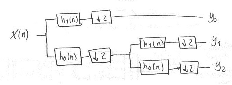
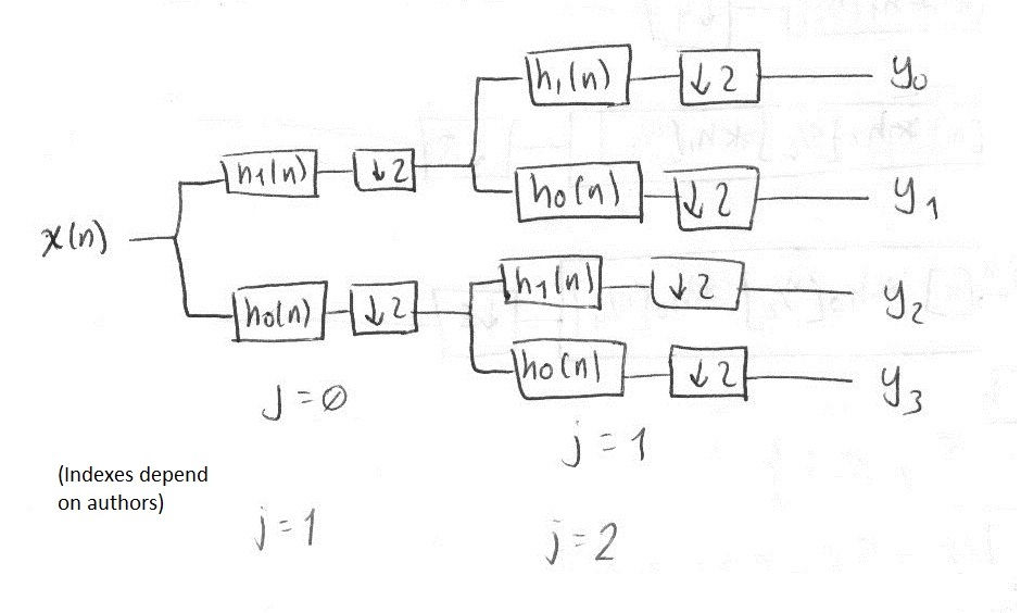
While DWT has a single "high-pass" branch that filters the signal with the h1 filter, the DWPT separates branches symmetricaly: this means that one gets equal frequency resolution for high and low parts of the signal.

There is also a "reverse-DWPT" filter structure, called Transmultiplexer (short TMX) that has its very own particular details, but I'll talk about it later, as it requires to understand well the programs used for DWT and DWPT.

A DWT filter bank sketch:

A DWPT filter bank sketch:

So, for a 2-level bank, DWT gets 3 branches (2 low-pass, 1 high-pass), while DWPT gets 4 (2 low-pass, 2 high-pass).

And, for a 3-level bank, DWT gets 5 branches (4 low-pass, 1 high-pass), while DWPT gets 8 (4 low-pass, 4 high-pass).

Noble identities

The mathematical tool we can use to reduce these equivalent filters is known as "Noble Identities", which can be reviewed in the following link:

http://cnx.org/content/m10432/latest/

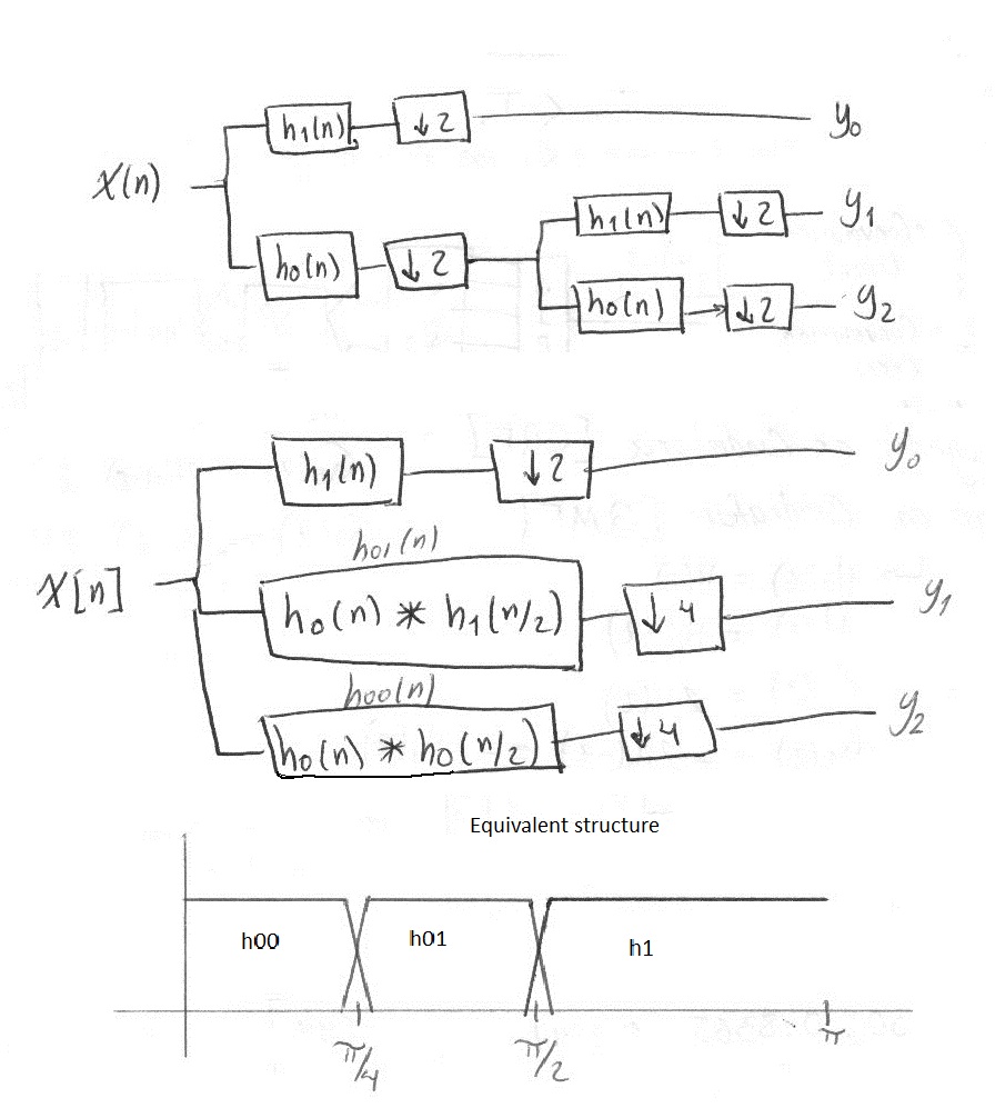
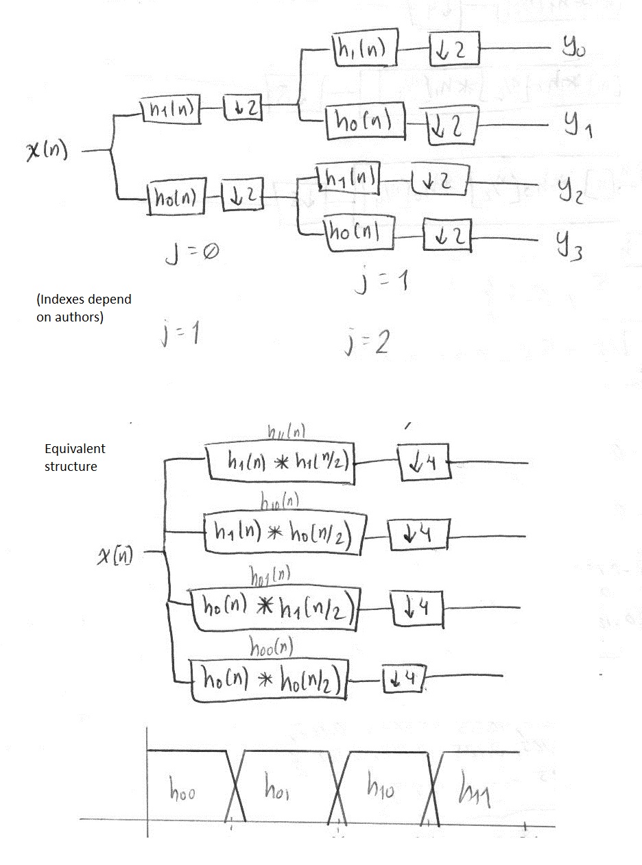
With this, one gets a filter that lets us do one single convolution instead of convoluting with each filter when moving along the branches. Simply put, it is faster and easier to compute.

First, a sketch on how the branches of a DWT filter bank look when converted to their equivalent pairs.

Then, a sketch on how the branches of a DWPT filter bank looks when converted to their equivalent pairs.

Result computation

Well, now we know how equivalent filters look like. Now, ¿How can we compute the results?

There are 2 possible ways of working this out:

1. With a convolution matrix (block processing)

2. Using chain-processing convolution

Convolution matrix (block processing)

In the first option one builds a matrix with the g or h filter coefficients, with a series of shiftings so that each output value is the sum of the products of each input value against its corresponding filter coefficient. This means, that for a given input of N samples, and a filter with L coefficients one must build a matrix of N columns with N+L-1 rows.

After that, multiply the input vector with the matrix and get the results. If the input has more samples, an even bigger matrix must be built. The problem here is that using a matrix the process gets very computing intensive, with all these sum and multiplication operations between vectors and matrices. It can work nicely with short filters, but as its lenght increases, the number of operation increases exponentially as the matrix grows.

When using a convolution matrix, one can use linear or circular convolution. Both options are implemented in code.

To see how a convolution matrix is built and how results are computed, check the code snippet at the bottom of this blog post.

Chain processing

On the other hand, another paradigm is to employ chain-processing, which is actually the most natural way to calculate a convolution. First, take the filter vector and transpose it, then sequentially multiply each of the filter's coefficients against the ones of the input, to get an output value. To get the remaining values, one must shift the input vector one position at a time.

This way, we can compute the transform of a real-time signal, when we don't know the size of the input (which we must know to build the matrix), as input data are taken sequentially.

Also -as we have seen before-, we have equivalent filters, this means that we only have to compute a single convolution and we're done. Furthermore, as there is a downsample stage, we only compute one of each N results (the one that we need), and therefore the computational time is greatly reduced against block (matrix) processing.

Later, I'll go into detail on how to work with chain processing, signaling rates, concurrency, synchronization (vital) and other programming issues I had to deal with.

In the meanwhile, you can check the code at the end of this blog post.

MATLAB Implementations (DWT, DWPT)

Summing up, the code for all the programs related to DWT, DWPT and TMX are listed below:

DWT - Linear convolution matrix: http://www.dsprelated.com/showcode/11.php

DWT - Circular convolution matrix: http://www.dsprelated.com/showcode/23.php

DWT - Linear Chain processing: http://www.dsprelated.com/showcode/47.php

Important, to run the DWT chain processing version you also need:

recorreder.m - http://www.dsprelated.com/showcode/43.php

formfilter.m (chain version) - http://www.dsprelated.com/showcode/44.php

formfilterdwt.m (chain version) - http://www.dsprelated.com/showcode/45.php

getsincdwt.m (chain version) - http://www.dsprelated.com/showcode/46.php

DWPT - Linear convolution matrix: coming soon!

DWPT - Circular convolution matrix: coming soon!

DWPT - Linear convolution Chain processing: coming soon!

Sign in