


Plotting Discrete-Time Signals
A discrete-time sinusoid can have frequency up to just shy of half the sample frequency. But if you try to plot the sinusoid, the result is not always recognizable. For example, if you plot a 9 Hz sinusoid sampled at 100 Hz, you get the result shown in the top of Figure 1, which looks like a sine. But if you plot a 35 Hz sinusoid sampled at 100 Hz, you get the bottom graph, which does not look like a sine when you connect the dots. We typically want the plot of a sampled sinusoid to resemble its continuous-time version. To achieve this, we need to interpolate (I discussed interpolation in my last post [1]).
In fact, we can design a general-purpose interpolator for plotting any sampled signal, as long as the signal’s bandwidth is less than some defined fraction of the Nyquist frequency fN = fs/2. A reasonable upper frequency for many applications is 0.8*fN, or 0.4*fs. A sinewave at 0.4*fs has 1/0.4 = 2.5 samples per cycle, or 5 samples every two cycles. If we interpolate it by 8, we will then have 20 samples/cycle. When we then connect these samples with straight lines, the plot looks to the eye like a smooth sinewave, as we’ll see.
The frequency response of an example interpolate-by-8 filter is shown in Figure 2. The filter is a linear-phase FIR lowpass, with passband of 0.4*fs and stopband of 0.6 *fs. We’ll use it in a Matlab function interp_by_8.m to interpolate some example signals. The Matlab function’s code is listed at the end of this article.
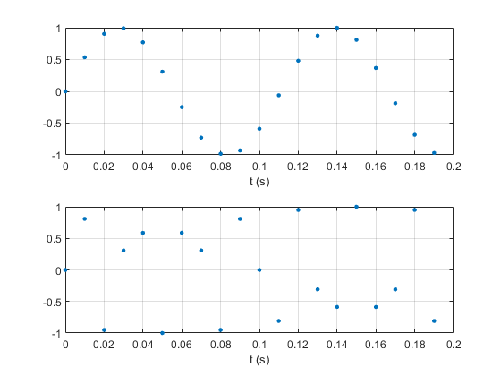
Figure 1. Sinusoids sampled at 100 Hz. Top: f0 = 9 Hz Bottom: f0 = 35 Hz.
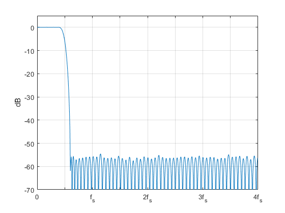
Figure 2. Interpolation-by-8 filter frequency response.
Example 1. Sinusoid
In this example, we’ll plot a 39 Hz sinusoid originally sampled at 100 Hz. Here is the Matlab code to create the signal and interpolate it to a sample rate of 800 Hz:
    fs= 100;                     % Hz sample frequency
    Ts= 1/fs;                    % s sample time
    N= 32;                       % number of samples
    n= 0:N-1;                    % time index of x
    f0= 39;                      % Hz frequency of sinusoid
    x= sin(2*pi*f0*n*Ts);        % sinusoid
    x_interp= interp_by_8(x);    % interpolated sinusoid
    %
    M= length(x_interp);
    m= 0:M-1;                    % time index of x_interp
    subplot(211),plot(n,x,'.','markersize',10),grid
    axis([0 32 -1 1]),xlabel('n')
    subplot(212),plot(m,x_interp,m(1:8:M),x_interp(1:8:M),'.',
    'markersize',10),grid
    axis([0 210 -1 1]),xlabel('m')
The original and interpolated signals are plotted in Figure 3. The interpolated signal shows the original sample times by plotting every 8th sample as an orange dot. The interpolated version includes an initial transient response of length equal to that of the interpolation filter (121 samples). The transient is due to the discontinuity at the start of the sine signal. The interpolator output is valid starting at m = 121.
This example poses the same display problem that comes up in digital oscilloscopes [2]. A scope might have a sinusoidal input at f0 = 390 MHz, sampled at fs = 1000 MHz. The scope uses interpolation to display the signal.
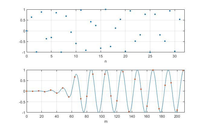
Figure 3. Top: Sinusoid with f0 = 39 Hz and fs = 100 Hz.
Bottom: Sinusoid interpolated by 8, with orange dot at every 8th sample.
Example 2. Filtered Pulse
In this example, x is a pulse signal filtered by a 3rd order Butterworth filter. The filter has a -3 dB frequency of 0.3*fs. The following Matlab code creates the pulse and then interpolates it by 8. Figure 4 shows x and the interpolated version. As before, the interpolated signal shows every 8th sample plotted as an orange dot.
    % 3rd order butterworth filter coeffs, fc/fs= 0.3
    % [b,a]= butter(3,2*.3)
    b= .2569*[1 3 3 1];
    a = [1 0.5772 0.4218 0.0563];
    u= [0 0 0 0 ones(1,12) zeros(1,10)];     % rectangular pulse
    x= filter(b,a,u);                        % filtered pulse signal
    x_interp= interp_by_8(x);                % interpolated signal
    N= length(x);
    n= 0:N-1;                                % time index of x
    M= length(x_interp);
    m= 0:M-1;                                % time index of x_interp
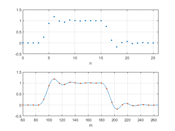
Figure 4. Top: Filtered pulse.
Bottom: Filtered pulse after interpolation by 8, with orange dot at every 8th sample.
Matlab Function interp_by_8.m
This Matlab function interpolates-by-eight a signal with bandwidth up to 0.4*fs. Note that we don’t need to know the sample frequency of the signal x to perform the interpolation. The only input to interp_by_8 is the vector x itself. See my last post [1] for a discussion of interpolation.
    % funtion interp_by_8.m  8/29/19 Neil Robertson
    % interpolation by 8 using 121-tap FIR filter
    % passband = 0 to 0.4*fs  stopband = 0.6 fs to 4fs
    %
    function x_interp= interp_by_8(x)
    b1= [-32 -12 -11 -6 2 12 22 31 37 38 33 20 2 -20 -43 -62 -74 -74 ...
       -62 -36 0 42 84 119 139 138 114 67 1 -74 -148 -207 -241 -239 ...
       -196 -114 -1 129 257 361 420 418 345 202 1 -234 -473 -676 ...
       -805 -822 -700 -426 -1 554 1205 1901 2586 3197 3681 3991];
    b= [b1 4098 fliplr(b1)]/2^15;    % interpolation filter coeffs
    N= length(x);
    x_up= zeros(1,8*N);
    x_up(1:8:end)= 8*x;              % upsampled signal
    x_interp= conv(x_up,b);          % interpolated signal
The FIR interpolation filter’s coefficients are plotted in Figure 5. In order to attenuate the images in the upsampled signal x_up, the filter’s stopband must start at 0.6 fs, where fs is the sample frequency of the interpolator’s input x. This is shown in figure 6, where the images of x_up’s spectrum are in orange. The filter’s frequency response magnitude is also plotted. The response in dB is plotted in Figure 2. Accuracy of interpolation depends on the filter’s passband flatness and stopband attenuation.
The filter coefficients were computed using the Parks-McClellan algorithm [3] as follows:
    Ntaps= 121;               % number of taps
    f= [0 .4 .6 4]/4;         % frequency vector relative to 4*fs
    a= [1 1 0 0];             % amplitude goal vector
    b= firpm(Ntaps-1,f,a);    % coefficients
    b= round(b*2^15)/2^15;    % quantized coefficients
The frequency vector f has passband of 0 to 0.4*fs and stopband of 0.6*fs to 4*fs. For example, if fs = 100 Hz (8*fs = 800 Hz), the passband is 0 to 40 Hz and the stopband is 60 to 400 Hz.
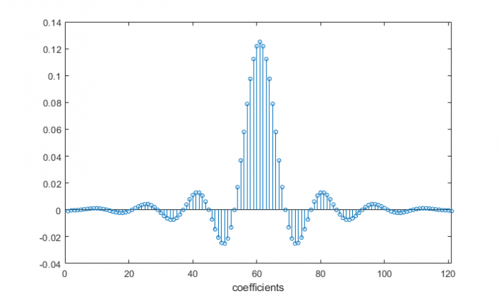
Figure 5. Coefficients of 121-tap interpolate-by-8 filter.
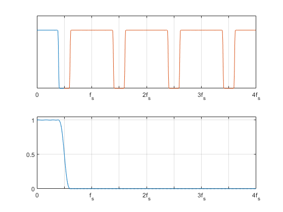
Figure 6. Top: Example spectrum of x_up occupying up to 0.4*fs, showing images beginning at 0.6 fs.
Bottom: Interpolation filter response (linear amplitude scale)
References
- Robertson, Neil, “Interpolation Basics”, DSP Related website, Aug, 2019, https://www.dsprelated.com/showarticle/1293.php
- AN1494, “Advantages and Disadvantages of Using DSP Filtering on Oscilloscope Waveforms”, Agilent (Keysight), 2004 http://literature.cdn.keysight.com/litweb/pdf/5989-1145EN.pdf
- The Mathworks website https://www.mathworks.com/help/signal/ref/firpm.html
Neil Robertson September, 2019
- Comments
- Write a Comment Select to add a comment

Hi Neil. Thanks for your blog and thanks for the Reference link to the interesting Keysight oscilloscope application note. Oscilloscopes sure have come a long way since the 300 kHz bandwidth Dumont scope I first touched in the late 1960s.

Hi Rick,
I noticed that Dumont was based in New Jersey, my home state. Did you use the scope with an HP audio generator?
Neil
Hi Neil. Ha ha. No, I didn't use an HP audio oscillator.
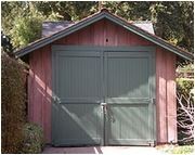
For you young folks out there, Neil is poking a little geriatric fun at me. His reference to an HP audio oscillator is, I think, referring to the famous audio oscillators that were the *very* first product of the Hewlett Packard company. Hewlett & Packard built their first audio oscillator in a garage in Palo Alta California in 1939. That garage is now listed on the National Register of Historic Places.
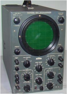
Actually, I used an HP audio oscillator in EE lab courses in the 1970's.
It looked like the example at this site:
Hi Neil. That's a neat photo. It's been a long time since I last saw "banana plugs" used as input connectors to a piece of equipment.
To post reply to a comment, click on the 'reply' button attached to each comment. To post a new comment (not a reply to a comment) check out the 'Write a Comment' tab at the top of the comments.
Please login (on the right) if you already have an account on this platform.
Otherwise, please use this form to register (free) an join one of the largest online community for Electrical/Embedded/DSP/FPGA/ML engineers:


