Determination of the transfer function of passive networks with MATLAB Functions

• Matlab
• DSPRelated
• Basics

With MATLAB functions, the transfer function of passive networks can be determined relatively easily. The method is explained using the example of a passive low-pass filter of the sixth order, which is shown in Fig.1

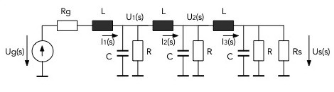
Fig.1 Passive low-pass filter of the sixth order

If one tried, as would be logical, to calculate the transfer function starting from the input, it would be quite complicated. On the other hand, if you start from the output, the determination of this function is simple and direct.

The output voltage is temporarily assumed to be known e.g. Us (s) = 1 and the input voltage Ug (s) that leads to this output voltage is calculated. Here the variable s  is the complex variable of the Laplace transform.

In MATLAB, the symbolic variable s is defined first.

s = tf('s');              % s as a symbolic variable of the Laplace transformation

% ------- Calculation of the transfer function starting from the output voltage

Us = 1;                       

I3 = Us*(1/Rs + 1/R + C*s);

U2 = I3*L*s + Us;

I2 = U2*(1/R + C*s) + I3;

U1 = I2*L*s + U2;

I1 = U1*(1/R + C*s) + I2;

Ug = I1*(L*s + Rg) + U1;

Hs = Us/Ug;

Then the currents and voltages are calculated according to the rules of the theory of electrical networks until you get to the input voltage. The complex impedance of a capacitance is 1 / (s*C) and that of an inductance is s*L Finally, the ratio of output voltage divided to input voltage leads to the desired transfer function in a symbolic form:

>> Hs

Hs =

                                                1

  ---------------------------------------------------------------------------------------------

  2.16e-46 s^6 + 1.476e-38 s^5 + 1.971e-30 s^4 + 9.551e-23 s^3 + 4.234e-15 s^2 + 1.15e-07 s    

                                                                                         + 1.13

Continuous-time transfer function.

Some MATLAB functions accept this symbolic object as arguments. As an example with step(Hs) and impulse(Hs) the step response and impulse response are determined and displayed.

The coefficients of the numerator and the denominator of the transfer function are extracted from the object H(s) as cell structures through:

[num, den] = tfdata (Hs);

Next are the numerical coefficients from the cells with

b = num {:};

a = the {:};

determined. The frequency response can now with the function freqs(b, a); be calculated and displayed.

The frequency response can also be determined numerically directly. First you choose the frequency range for the frequency response. For this network one can choose two decades on the left to two decades on the right of the characteristic frequency. The characteristic frequency is the resonance frequency of a section of the filter:

w0 = 1 / sqrt (L * C);     % Resonance frequency of a stage (rad / s)

f0 = w0 / (2 * pi); % Hz

The frequency range is then selected with the following instructions:

f = logspace (round (log10 (f0 / 100)), round (log10 (f0 * 100)), 200);

          % Frequency range with 2 decades left and right

          % of the resonance frequency

The complex variables of the network are then determined directly numerically, similar to the previous one:

% ------- 2nd variant

omega = 2 * pi * f;           % Frequency range (rad / s)

% ------- Calculation of the transfer function based on the output

Us = 1;                            % Output voltage

% Us = 1 * exp(j * pi / 3);            % Any other output voltage

I3 = Us * (1 / Rs + 1 / R + C * j * omega);

U2 = I3. * (L * j * omega) + Us;

I2 = U2. * (1 / R + C * j * omega) + I3;

U1 = I2. * (L * j * omega) + U2;

I1 = U1. * (1 / R + C * j * omega) + I2;

Ug = I1. * (L * j * omega + Rg) + U1;

Hs2 = Us./Ug; % Transfer function

For the following network parameters

Rg = 100; % Output resistance of the source

L = 30e-6; % Inductance

C = 20e-12; % Capacity

R = 10e3; % Loss Resistance of Capacitance

Rs = 1000; % Load resistance

the amplitude response is shown in Fig. 2

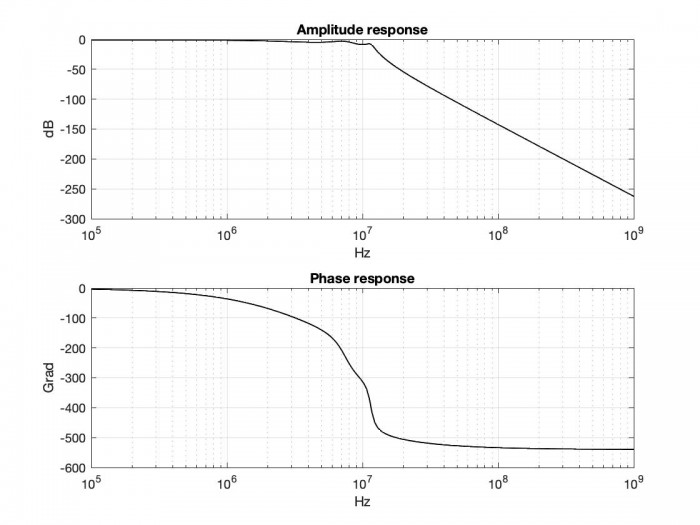
Fig. 2 Frequency response of the network

In the MATLAB statements shown, the point in front of the operation sign causes the element white operation. As an example in

U1 = I2. * (L * j * omega) + U2;

shows (. *) the element-white multiplication of the vector I2 by the vector L * j * omega.

The transfer_1.m script from the file with the same name also examines other properties of the network that are no longer discussed here.

The file transfer_1.m is given in the appendix.

transfer_1.m

Sign in