Interpolator Design: Get the Stopbands Right

• Matlab
• Multirate DSP
• Tutorials

Designing an interpolator needn’t be confusing.  In this article, I’ll present a simple approach for designing interpolators that takes the guesswork out of determining the stopbands (For a basic introduction to interpolators, see my earlier post [1]).

Figure 1a shows a block diagram of an interpolator, which consists of an up-sampler that increases the sample rate of the input signal x by an integer factor of L, and a Finite Impulse Response (FIR) low-pass filter (LPF).  The design problem is to find an efficient design of the LPF:  this requires defining the filter’s stopbands based on the images of the up-sampled signal.  While this may sound like a chore, you don’t really need to apply that much mental exertion to determine the images.  Here is a simple method to find the images and design the LPF:

1. Up-sample the interpolator’s input signal x, as shown in Figure 1b.
2. Take the DFT of the up-sampler output x_up.  Plot the DFT magnitude to reveal the images of x_up.
3. Define a magnitude response goal function for the LPF based on the spectral plot.
4. Design the LPF using the Parks-McLellan algorithm [2] (e.g., by using the Matlab function firpm [3]).

The remainder of this article is an example that illustrates these steps.

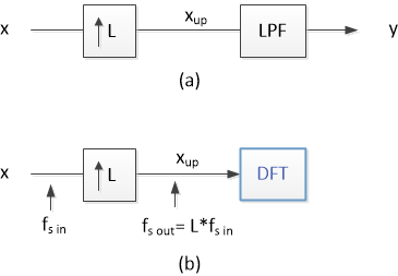
Figure 1.  a)  Interpolator block diagram.  b)  Finding the spectrum of the up-sampler’s output x_up.

Example – QAM Modulator

Figure 2a shows a block diagram of the digital filters used in a Quadrature Amplitude Modulator (QAM) [4].  Each I or Q path consists of an FIR pulse-shaping filter, followed by an interpolator.  To begin with, we need to obtain the interpolator input signal x.  If we apply an impulse to the I or Q input, x is simply the impulse response (i.e., the coefficients) of the pulse shaping filter, as shown in Figure 2b.  We can then perform up-sampling and compute the DFT of x_up.

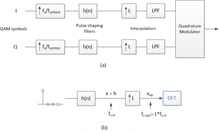
Figure 2.  a) Block diagram of QAM modulator’s pulse shaping filter and interpolator.

                b) Finding the spectrum of x_up for interpolator input x = h.

For this example, let the interpolator’s input sample rate fs_in = 4 MHz and let L = 5.  Thus, output sample rate is 20 MHz, and the modulated QAM signal falls between 0 and 10 MHz.  Sample rates and the pulse-shaping filter coefficients h are listed in the following Matlab code.  The pulse-shaping filter has -3 dB bandwidth of 0.5 MHz.  The coefficients were generated using the method described in an earlier post [5].

    fs_in= 4;            % MHz interpolator input sample rate
    L= 5;                % upsample ratio
    fs_out= L*fs_in;     % MHz interpolator output sample rate
    % 63-tap Pulse-shaping filter coefficients (impulse response)
    % Root-Nyquist, 4 samples/symbol, excess bw = 0.3
    u= [2 -1 -4 -6 -3 5 13 15 4 -16 -32 -30 -1 40 66 49 -13 ...
       -88 -121 -71 53 180 213 91 -153 -381 -409 -106 519 1285 1915];
    h= [u 2159 fliplr(u)]/2^13;
    x= h;                % interpolator input signal

Next, we up-sample x by L = 5.  Normally, the up-sampler has a gain of L to achieve interpolator output level equal to input level.  Since our goal is just to find the spectrum, we omit the scaling.

    % upsampling
    x_up= zeros(1,length(x)*L);
    x_up(1:L:length(x)*L)= x;      % note: omitted scaling by L

x and a portion of x_up are plotted in Figure 3.  We now compute the spectrum of x_up using the DFT, and generate a discrete frequency vector to use as a frequency axis:

    % compute spectrum of x_up
    N= 2048;                      % number of frequency samples
    X_up= fft(x_up,N);
    X_updB= 20*log10(abs(X_up));  % dB-magnitude spectrum of x_up
    k= 0:N-1;                     % frequency index
    f= k*fs_out/N;                % MHz discrete frequency vector

The spectrum of x is plotted in the top graph of Figure 4, and the spectrum of x_up is plotted over f = 0 to fs_out in the bottom graph.  This spectrum has images centered at multiples of fs_in = 4 MHz.

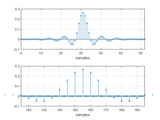
Figure 3. Top:  Interpolator input signal x.

Bottom:  Center portion of up-sampler output signal x_up (omitting amplitude scaling by L).

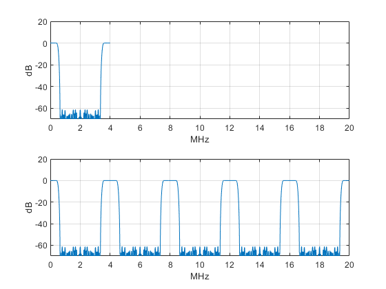
Figure 4. Top:  Spectrum of x over f = 0 to fs_in = 4 MHz.

Bottom:  Spectrum of x_up over f = 0 to fs_out = 20 MHz.

Now we’re ready to define the magnitude response goal function for the LPF.  Figure 5 (top) again shows the spectrum of x_up, this time plotted over f = 0 to fs_out/2.  The dots on the plot indicate the edge of the passband and the edges of the two stopbands that are needed to attenuate the spectral images.  The passband edge is at 0.62 MHz, which is high enough to minimize amplitude roll-off over the signal’s bandwidth.

Figure 5 (bottom) shows the goal function for the LPF.  As shown, the magnitude response goal is 1.0 in the passband and 0.0 in the stopbands.  The response is unspecified in the other frequency ranges.

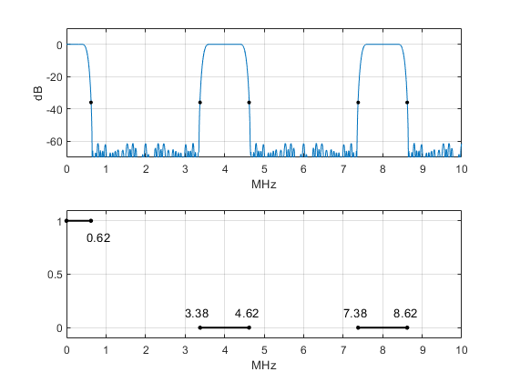
Figure 5. Top:  Spectrum of x_up over f = 0 to fs_out/2, showing frequencies (MHz) for goal function.

Bottom:  Magnitude response goal function for interpolator LPF.

Now, at last, we can synthesize the interpolator’s LPF.  The following Matlab code uses function firpm to synthesize the filter via the Parks-McClellan algorithm. We’ll synthesize a filter of order 24 (25 taps).  The inputs to firpm are filter order, a vector of normalized frequencies, and a vector of goal function values at each frequency.  After finding the coefficients, we compute the magnitude response of the LPF via the DFT.

    % synthesize interpolator LPF using Parks-McClellan algorithm
    ff= [0 .62 3.38 4.62 7.38 8.62]/(fs_out/2);   % normalized freq vector
    a=  [1  1   0    0     0    0];               % magnitude response goal vector
    ntaps= 25;
    b= firpm(ntaps-1,ff,a);                      % Parks-McClellan filter synthesis
    b= round(b*2^14)/2^14;                       % quantize coefficients
    % compute LPF magnitude response
    N= 2048;                                     % number of frequency samples
    H= fft(b,N);
    HdB= 20*log10(abs(H));                       % dB-magnitude response vector
    k= 0:N-1;                                    % frequency index
    f= k*fs_out/N;                               % MHz discrete frequency vector

The interpolator output y is simply the convolution of x_up, which we computed earlier, and the LPF coefficients b:

    % compute interpolator output y
    y= conv(x_up,b);

Figure 6 shows the performance of the LPF.  The top plot is the spectrum of x_up, the middle plot shows the LPF magnitude response, and the bottom plot shows the spectrum of the interpolator’s output y.  Note in the LPF magnitude response how the attenuation is high in the specified stopbands and lower in the unspecified frequency ranges.  The time-domain interpolator input and output signals are shown in Figure 7 (The output signal is scaled by L = 5, as compensation for omitting scaling in the up-sampler).

Was it worth the effort to define the two stopbands in this way?  We could have defined a goal function with a single stopband from 3.38 MHz to 10 MHz as follows:

    % single stopband case
    ff= [0 .62 3.38 10]/(fs_out/2);     % normalized frequency vector
    a=  [1   1  0   0 ];                % magnitude response goal vector

Figure 8 compares the magnitude response of the two filter synthesis cases for ntaps = 25.  The two-stopband filter has about 10 dB more attenuation than the single-stopband case – a significant advantage.  Regarding hardware implementation, the interpolator can be implemented efficiently using a polyphase design [6,7,8].

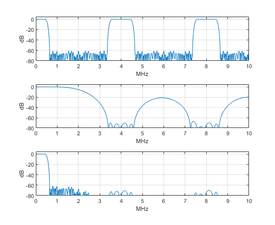
Figure 6.  Interpolator LPF performance.  Top:  Spectrum of x_up over f = 0 to fs_out/2.

Middle:  Magnitude response of LPF.    Bottom:  Spectrum of interpolator output y.

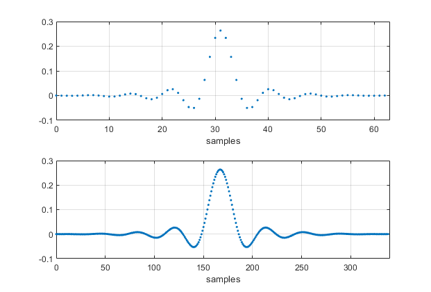
Figure 7.  Top:  Interpolator input signal x.   Bottom:  Interpolator output signal y (scaled by L = 5).

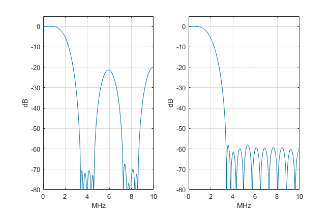
Figure 8.  Magnitude responses of 25-tap LPF’s for different goal functions.

Left:  using a goal function with two stopbands.

Right:  using a goal function with a single stopband.

References

1.  Robertson, Neil, “Interpolation Basics”, DSPrelated website, Aug, 2019, https://www.dsprelated.com/showarticle/1293.php

2.  Lyons, Richard, Understanding Digital Signal Processing, 3^rd Ed., Pearson, 2011, section 5.6

3.  Mathworks website, firpm, https://www.mathworks.com/help/signal/ref/firpm.html

4.  Rice, Michael, Digital Communications, A Discrete-Time Approach, Pearson, 2009, Section 10.1.1.

5.  Robertson, Neil, “Design Square-Root Nyquist Filters”, DSPrelated website, July, 2020, https://www.dsprelated.com/showarticle/1361.php

6.  Lyons, section 10.10

7.  harris, fredric j., Multirate Signal Processing, Pearson, 2004, section 7.2.

8.  Mitra, Sanjit K., Digital Signal Processing, 2^nd Ed., McGraw Hill, 2001, section 10.4.

                            Neil Robertson             July, 2023          Revised 7/12/23

Sign in