My FFT code uses CMSIS DSP function arm_biquad_cascade_df1_f32() with coefficients set up for 12kHz, sample rate 48k, 60dB stopband, elliptic.

I know the original developer used Iowa Hills filter designer, but that's disappeared from the Internet.

I've tried to use BiQuadDesigner (arachnoid.com) to do this, but it doesn't seem to work with the 192 KHz sample rate I'm now using, so I need to recreate the same filter at 750Hz, 1.5KHz, 3, 6, 12 and 24KHz.

These filters seem to work or do no harm with the 192KHz samples, but I'd like to test with the correct values for 192KHz sampling.

The developer commented below "a1 and coeffs[A2] negated!", any ideas why?

Thanks, Rob

        (float32_t*)(const float32_t[]) {

            // 2x magnify - index 1

            // 12kHz, sample rate 48k, 60dB stopband, elliptic

            // a1 and coeffs[A2] negated! order: coeffs[B0], coeffs[B1], coeffs[B2], a1, coeffs[A2]

            // Iowa Hills IIR Filter Designer

            0.228454526413293696,

            0.077639329099949764,

            0.228454526413293696,

            0.635534925142242080,

            -0.170083307068779194,

            0.436788292542003964,

            0.232307972937606161,

            0.436788292542003964,

            0.365885230717786780,

            -0.471769788739400842,

            0.535974654742658707,

            0.557035600464780845,

            0.535974654742658707,

            0.125740787233286133,

            -0.754725697183384336,

            0.501116342273565607,

            0.914877831284765408,

            0.501116342273565607,

            0.013862536615004284,

            -0.930973052446900984

        },

Hi Robmar,

a biquad has 3 forward coffs and 2 feedback coffs, so your 20 coffs are 4 biquad filters. I analyzed them with Matlab and they really constitute a nice 60db halfband filter, 12kHz stopband at 48kHz/2 Nyquist. The feedback coffs are negated indeed.

This is the frequency response of the filter.

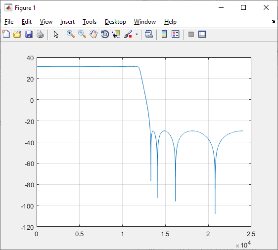
Your pole/zero setup is centered around 90° on the unit circle, because Nyquist 24kHz is at 180°, so your stop frequency 12kHz is at 90° angle. 

Your new new sample freq ist 192kHz, stop frequency still at 12khz. So your pole/zero setup is centered at 180°/8 = 22.5°. You rotate the poles/zeros by 90°-22.5°.

That is the result

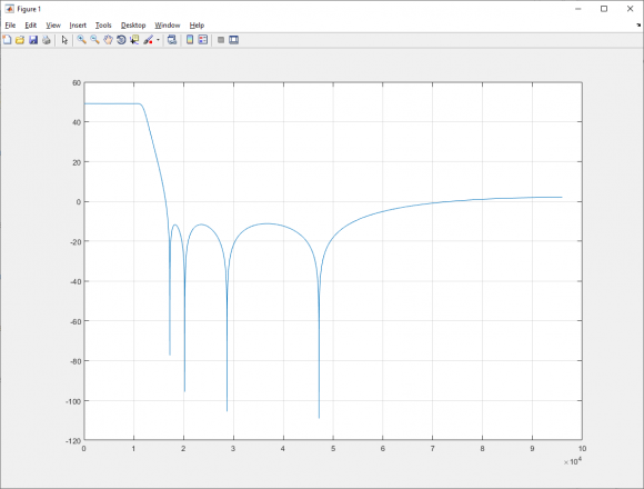
For high frequencies attenuation reduces to 50dB. You mitigate this by pushing the zeros higher up.

New coefficients and Matlab code enclosed.

big fun

Cheers Detlef

0.22845453
-0.38627877
0.22845453
0.72895199
-0.17008331
0.43678829
-0.68911864
0.43678829
1.36331536
-0.47176979
0.53597465
-0.63296952
0.53597465
1.64914965
-0.93097305
0.50111634
-0.02797031
0.50111634
1.78810523
-0.93097305

clear

fb1=[0.228454526413293696,0.077639329099949764,0.228454526413293696];
fa1=-[-1 ,0.635534925142242080,-0.170083307068779194];
fb2=[0.436788292542003964,0.232307972937606161,0.436788292542003964];
fa2=-[ -1, 0.365885230717786780,-0.471769788739400842];
fb3=[0.535974654742658707,0.557035600464780845,0.535974654742658707];
fa3=-[-1 0.125740787233286133,-0.754725697183384336];
fb4=[0.501116342273565607,0.914877831284765408, 0.501116342273565607];
fa4=-[-1 0.013862536615004284,-0.930973052446900984];

fb=poly([roots(fb1) ;roots(fb2);roots(fb3);roots(fb4)] )
fa=poly([roots(fa1) ;roots(fa2);roots(fa3);roots(fa4)] )
H=freqz(fb,fa,24000);

plot(20*log10(abs(H)));

c= exp(j*(-pi*(90-22.5)/180));
fb1mod=fb1(1)*poly([c; conj(c)].*roots(fb1));
fb2mod=fb2(1)*poly([c; conj(c)].*roots(fb2));
fb3mod=fb3(1)*poly([c; conj(c)].*roots(fb3));
fb4mod=fb4(1)*poly([c; conj(c)].*roots(fb4));
fa1mod=       poly([c; conj(c)].*roots(fa1));
fa2mod=       poly([c; conj(c)].*roots(fa2));
fa3mod=       poly([c; conj(c)].*roots(fa3));
fa4mod=       poly([c; conj(c)].*roots(fa4));

fbmod=poly([roots(fb1mod) ;roots(fb2mod);roots(fb3mod);roots(fb4mod)] )
famod=poly([roots(fa1mod) ;roots(fa2mod);roots(fa3mod);roots(fa4mod)] )
Hmod=freqz(fbmod,famod,96000);

plot(20*log10(abs(Hmod)));

disp(sprintf('%.8f',fb1mod(1)))
disp(sprintf('%.8f',fb1mod(2)))
disp(sprintf('%.8f',fb1mod(3)))
disp(sprintf('%.8f',-fa1mod(2)))
disp(sprintf('%.8f',-fa1mod(3)))

disp(sprintf('%.8f',fb2mod(1)))
disp(sprintf('%.8f',fb2mod(2)))
disp(sprintf('%.8f',fb2mod(3)))
disp(sprintf('%.8f',-fa2mod(2)))
disp(sprintf('%.8f',-fa2mod(3)))

disp(sprintf('%.8f',fb3mod(1)))
disp(sprintf('%.8f',fb3mod(2)))
disp(sprintf('%.8f',fb3mod(3)))
disp(sprintf('%.8f',-fa3mod(2)))
disp(sprintf('%.8f',-fa4mod(3)))

disp(sprintf('%.8f',fb4mod(1)))
disp(sprintf('%.8f',fb4mod(2)))
disp(sprintf('%.8f',fb4mod(3)))
disp(sprintf('%.8f',-fa4mod(2)))
disp(sprintf('%.8f',-fa4mod(3)))

return

Wow, thanks Detlef, that looks good I will try those values and let you know how they work.

As I've upped the sample rate to 192KHz, the code handles 96 and 192 KHz bandwidths, could you use your setup to produce the values for those too?

Rob

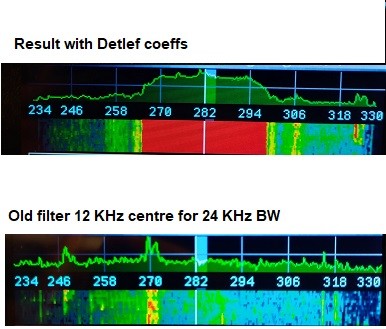
Hi Ketlef, here we see using your coeffs with the 96 KHz scope view, we can see the cutoff is spot on from 270 to 294 KHz, so that's 24 KHz!

Using the old 24 KHz sample rate filter for the 96KHz scope doesn't seem to filter at all with the 192KHz samples.

Any ideas why the level so much higher on the scope with your coeefs, like more noise or something? (Edit: Dooh, of course the lower areas are show attenuated, as per the filter design)

Hi,

I do not know what you are doing. Is it the 'audacity' app ? What is '96kHz scope view'?

lost

Detlef

It's a spectrum display with waterfall, the spectrum is shown at top as the magnitude of the signals across the bandwidth.

This is a very common application using FFT from the CMSIS DSP library for Arm CPUs, most devices use the same coding.

Your values need to be in the same format as the list I published, with "// a1 and coeffs[A2] negated!"

Hi

>>>>>>

They are, take a look at the Matlab Code.

So its a Waterfall spectrum !?

- What input signal?  Speech, broadband, real artificial ?

- Analog, digital?

- Samplerate, if analog?

- Window width ? Window type?

- scaling of the x-axis ('294kHz is 24kHz' ????)

- scaling of the y-axis. dB? Looks like a bandpass, I designed a lowpass.

Cheers Detlef

Yes, input is IQ signals, can be from audio, from a quadrature mixer, usually radio and voice.

Sample rate is 192 KHz, but Nyquist limit apart, the spectrum produced over 192 KHz is quite free of aliases, which only occur every 192 KHz, so its quite useable.

Hann.

Scaling 192 KHz, 96 KHz, 48 Khz, 24... 3, zoom selection.

20 dB vertical height.

Would be interesting to try coefficients for a 192 KHz band pass filter with this setup, see how it looks, maybe it will help with the aliases.

Rob

Hi,

the coefficients will work for 192kHz samplerate, 12khz cutoff, I guarantee. For 192kHz samplerate you may not have any frequency above 96kHz, not 192khz. Check out the filter with an appropriate, known input signal, a clean sinewave for instance.

Cheers

Detlef

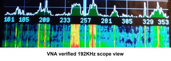
Hey, I use a nanoVNA for testing, great little devices! :D

As shown in the image I posted, your filter produces a hump across the 24KHz bandwidth, and there are signals showing on either side that haven't been attenuated, so something must be off.

Any idea what could cause that?  I mean the magnitudes in the bins should't be increased, and there should be -50dB attenuation either side, so looks like somethings up, but what?

Here's an image from the unit working, cheers n beers, Rob

Rob

Hi Detlef, it just clicked that the image using the filter coefficients you produced is correct, the attenuation shows as around -40dB on the screenshot I posted, hence the hump!

Would you mind sharing a link with me for the application you used?

Cheers, Rob

Hi, as I mentioned, I used Matlab.

Cheers Detlef

In most depictions of the standard forms, the feedback coefficients are negated. This is just convenient convention based on how the transfer function as given maps to the implementation: if the denominator coefficient is described with a positive quantity (such as $1+ a1 z^{-1}$, -a1 is what is actually used for the feedback. 

Do you know the Iowa Hills filter designer application, or something similar perhaps?

If you have access to matlab use matlab to design the prototype filter, the use matlab's command tf2sos. see below! when using this script you may want to redistribute gain scaling factor (G) over the separate 2nd order segments 

ellip Elliptic or Cauer digital and analog filter design.

    [B,A] = ellip(N,Rp,Rs,Wp) designs an Nth order lowpass digital elliptic

    filter with Rp decibels of peak-to-peak ripple and a minimum stopband

    attenuation of Rs decibels. ellip returns the filter coefficients in

    length N+1 vectors B (numerator) and A (denominator). The passband-edge

    frequency Wp must be 0.0 < Wp < 1.0, with 1.0 corresponding to half the

    sample rate.  Use Rp = 0.5 and Rs = 20 as starting points, if you are

    unsure about choosing them.

tf2sos Transfer Function to Second Order Section conversion.

    [SOS,G] = tf2sos(B,A) finds a matrix SOS in second-order sections 

    form and a gain G which represent the same system H(z) as the one

    with numerator B and denominator A.  The poles and zeros of H(z)

    must be in complex conjugate pairs. 

    SOS is an L by 6 matrix with the following structure:

        SOS = [ b01 b11 b21  1 a11 a21 

                b02 b12 b22  1 a12 a22

                ...

                b0L b1L b2L  1 a1L a2L ]

    Each row of the SOS matrix describes a 2nd order transfer function:

                  b0k +  b1k z^-1 +  b2k  z^-2

        Hk(z) =  ----------------------------

                   1 +  a1k z^-1 +  a2k  z^-2

    where k is the row index.

    G is a scalar which accounts for the overall gain of the system. If

    G is not specified, the gain is embedded in the first section. 

    The second order structure thus describes the system H(z) as:

        H(z) = G*H1(z)*H2(z)*...*HL(z)

Thanks very much, but I'm really hoping for something like Iowa Hills filter designer, which unfortunately has disappeared.

You may check this:

https://developer.arm.com/documentation/102463/lat...

This is an example of the cmsis python wrapper, it also uses an biquad cascaded df1 filter (arm_biquad_casd_df1_inst_q31()). 

Filter design is done in python. The b-coeffs need to be negated. In the example this is done by:

coefs=np.reshape(np.hstack((sos[:,:3],-sos[:,4:])),15)

These coefs can then be used with

arm_biquad_cascade_df1_init_f32()

Hi, thanks for that, looks interesting, though I'm not that familiar with Python.  How long would it take you to do, guessing you know Python well

If you are familiar with matlab, I don't think it is a big deal. However, tool setup will take some time (python, ide,...) 

Another tool I use on a occasionally basis is pyfda. It's a filter design GUI much like Matlab Filter Design Toolbox but written in python. 

https://github.com/chipmuenk/pyfda

There are also binaries. No need for a full python dev setup. 

Time I'm short on, hence looking for a helping hand, or a filter design tool like Iowa Hills. Maybe someone has a copy?...

Did you check the pydfa tool? From my pov, that is exactly what you're asking for: 

A filter design GUI

Thanks for the tip, looks great but they don't make it easy, no runnable binary is available

Mmh, 

I cite the Installation.md:

The executable is operating system specific, I can only provide exectuables for Windows 10 and for the version of my currently installed Linux distro. This may or may not work on your Linux distro, please try.

Here is a direct link to the releases:

Executables for win and osx. 

I missed that, thanks for pointing it out.

Thanks, maybe you could give it a go, and I´ll plug your data in, see how it runs

Think of the biquad definition:

( a0 * y[n] ) + ( a1 * y[ n - 1 ] ) + ( a2 * y[ n - 2 ] ) =

 ( b0 * x[n] ) + ( b1 * x[ n - 1 ] ) + ( b2 * x[ n - 2 ] )

So, with a0 = 1, the value of y[n] is:

y[n] = ( -a1 * y[ n - 1 ] ) + ( -a2 * y[ n - 2 ] ) + ( b0 * x[ n ] ) + ( b1 * x [ n - 1 ] + ( b2 * x[ n - 2 ) 

That, I suspect, is the reason for the negation of the "a" coefficients.

Robert Wolfe