


The Four Direct Forms
Direct-Form I
As mentioned in §5.5,
the difference equation
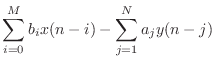 |
(10.1) |
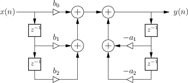
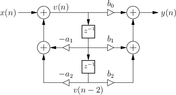
specifies the Direct-Form I (DF-I) implementation of a digital filter [60]. The DF-I signal flow graph for the second-order case is shown in Fig.9.1.
The DF-I structure has the following properties:
- It can be regarded as a two-zero filter section followed in series
by a two-pole filter section.
- In most fixed-point arithmetic schemes (such as two's complement,
the most commonly used
[84]10.1)
there is no possibility of internal filter overflow. That is,
since there is fundamentally only one summation point in the filter,
and since fixed-point overflow naturally ``wraps around'' from the
largest positive to the largest negative number and vice versa, then
as long as the final result
 is ``in range'', overflow is
avoided, even when there is overflow of intermediate results in the sum
(see below for an example). This is an important, valuable, and
unusual property of the DF-I filter structure.
is ``in range'', overflow is
avoided, even when there is overflow of intermediate results in the sum
(see below for an example). This is an important, valuable, and
unusual property of the DF-I filter structure.
- There are twice as many delays as are necessary. As a result,
the DF-I structure is not canonical with respect to delay. In
general, it is always possible to implement an
 th-order filter
using only delay elements.
th-order filter
using only delay elements.
- As is the case with all direct-form filter structures
(those which have coefficients given by the transfer-function coefficients),
the filter poles and zeros can be very sensitive to round-off errors
in the filter coefficients. This is usually not a problem for a
simple second-order section, such as in Fig.9.1, but it can
become a problem for higher order direct-form filters. This is the
same numerical sensitivity that polynomial roots have with respect to
polynomial-coefficient round-off. As is well known, the sensitivity
tends to be larger when the roots are clustered closely together, as
opposed to being well spread out in the complex plane
[18, p. 246]. To minimize this sensitivity, it is common to
factor filter transfer functions into series and/or parallel second-order
sections, as discussed in §9.2 below.
It is a very useful property of the direct-form I implementation that it cannot overflow internally in two's complement fixed-point arithmetic: As long as the output signal is in range, the filter will be free of numerical overflow. Most IIR filter implementations do not have this property. While DF-I is immune to internal overflow, it should not be concluded that it is always the best choice of implementation. Other forms to consider include parallel and series second-order sections (§9.2 below), and normalized ladder forms [32,48,86].10.2Also, we'll see that the transposed direct-form II (Fig.9.4 below) is a strong contender as well.
Two's Complement Wrap-Around
In this section, we give an example showing how temporary overflow in two's complement fixed-point causes no ill effects.
In 3-bit signed fixed-point arithmetic, the available numbers are as shown in Table 9.1.
|
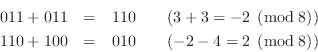
Let's perform the sum ![]() , which gives a temporary overflow
(
, which gives a temporary overflow
(![]() , which wraps around to
, which wraps around to ![]() ), but a final result (
), but a final result (![]() ) which
is in the allowed range
) which
is in the allowed range ![]() :10.3
:10.3
Now let's do ![]() in three-bit two's complement:
in three-bit two's complement:
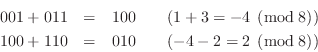
In both examples, the intermediate result overflows, but the final result is correct. Another way to state what happened is that a positive wrap-around in the first addition is canceled by a negative wrap-around in the second addition.
Direct Form II
The signal flow graph for the Direct-Form-II (DF-II) realization of the second-order IIR filter section is shown in Fig.9.2.
The difference equation for the second-order DF-II structure can be written as
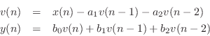
which can be interpreted as a two-pole filter followed in series by a two-zero filter. This contrasts with the DF-I structure of the previous section (diagrammed in Fig.9.1) in which the two-zero FIR section precedes the two-pole recursive section in series. Since LTI filters in series commute (§6.7), we may reverse this ordering and implement an all-pole filter followed by an FIR filter in series. In other words, the zeros may come first, followed by the poles, without changing the transfer function. When this is done, it is easy to see that the delay elements in the two filter sections contain the same numbers (see Fig.5.1). As a result, a single delay line can be shared between the all-pole and all-zero (FIR) sections. This new combined structure is called ``direct form II'' [60, p. 153-155]. The second-order case is shown in Fig.9.2. It specifies exactly the same digital filter as shown in Fig.9.1 in the case of infinite-precision numerical computations.
In summary, the DF-II structure has the following properties:
- It can be regarded as a two-pole filter section followed by a two-zero
filter section.
- It is canonical with respect to delay. This happens because
delay elements associated with the two-pole and two-zero sections are
shared.
- In fixed-point arithmetic, overflow can
occur at the delay-line input (output
of the leftmost summer in Fig.9.2), unlike in the DF-I
implementation.
- As with all direct-form filter structures, the poles
and zeros are sensitive to round-off errors in the coefficients
 and
and  , especially for high transfer-function orders. Lower
sensitivity is obtained using series low-order sections (e.g., second
order), or by using ladder or lattice filter structures
[86].
, especially for high transfer-function orders. Lower
sensitivity is obtained using series low-order sections (e.g., second
order), or by using ladder or lattice filter structures
[86].
More about Potential Internal Overflow of DF-II
Since the poles come first in the DF-II realization of an IIR filter,
the signal entering the state delay-line (see Fig.9.2) typically
requires a larger dynamic range than the output signal ![]() . In
other words, it is common for the feedback portion of a DF-II IIR
filter to provide a large signal boost which is then
compensated by attenuation in the feedforward portion (the
zeros). As a result, if the input dynamic range is to remain
unrestricted, the two delay elements may need to be implemented with
high-order guard bits to accommodate an extended dynamic range.
If the number of bits in the delay elements is doubled (which still
does not guarantee impossibility of internal overflow), the benefit of
halving the number of delays relative to the DF-I structure is
approximately canceled. In other words, the DF-II structure, which is
canonical with respect to delay, may require just as much or more
memory as the DF-I structure, even though the DF-I uses twice as many
addressable delay elements for the filter state memory.
. In
other words, it is common for the feedback portion of a DF-II IIR
filter to provide a large signal boost which is then
compensated by attenuation in the feedforward portion (the
zeros). As a result, if the input dynamic range is to remain
unrestricted, the two delay elements may need to be implemented with
high-order guard bits to accommodate an extended dynamic range.
If the number of bits in the delay elements is doubled (which still
does not guarantee impossibility of internal overflow), the benefit of
halving the number of delays relative to the DF-I structure is
approximately canceled. In other words, the DF-II structure, which is
canonical with respect to delay, may require just as much or more
memory as the DF-I structure, even though the DF-I uses twice as many
addressable delay elements for the filter state memory.
Transposed Direct-Forms
The remaining two direct forms are obtained by formally transposing direct-forms I and II [60, p. 155]. Filter transposition may also be called flow graph reversal, and transposing a Single-Input, Single-Output (SISO) filter does not alter its transfer function. This fact can be derived as a consequence of Mason's gain formula for signal flow graphs [49,50] or Tellegen's theorem (which implies that an LTI signal flow graph is interreciprocal with its transpose) [60, pp. 176-177]. Transposition of filters in state-space form is discussed in §G.5.
The transpose of a SISO digital filter is quite straightforward to find: Reverse the direction of all signal paths, and make obviously necessary accommodations. ``Obviously necessary accommodations'' include changing signal branch-points to summers, and summers to branch-points. Also, after this operation, the input signal, normally drawn on the left of the signal flow graph, will be on the right, and the output on the left. To renormalize the layout, the whole diagram is usually left-right flipped.
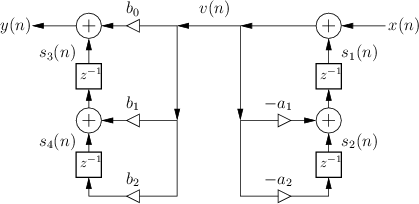
Figure 9.3 shows the Transposed-Direct-Form-I (TDF-I) structure for the general second-order IIR digital filter, and Fig.9.4 shows the Transposed-Direct-Form-II (TDF-II) structure. To facilitate comparison of the transposed with the original, the inputs and output signals remain ``switched'', so that signals generally flow right-to-left instead of the usual left-to-right. (Exercise: Derive forms TDF-I/II by transposing the DF-I/II structures shown in Figures 9.1 and 9.2.)
 |
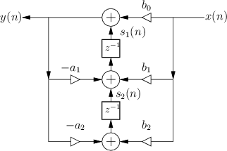 |
Numerical Robustness of TDF-II
An advantage of the transposed direct-form II structure (depicted in
Fig.9.4) is that the zeros effectively precede the poles in
series order. As mentioned above, in many digital filters design, the
poles by themselves give a large gain at some frequencies, and the
zeros often provide compensating attenuation. This is especially true
of filters with sharp transitions in their frequency response, such as
the elliptic-function-filter example on page ![]() ; in such
filters, the sharp transitions are achieved using near pole-zero
cancellations close to the unit circle in the
; in such
filters, the sharp transitions are achieved using near pole-zero
cancellations close to the unit circle in the ![]() plane.10.4
plane.10.4
Next Section:
Series and Parallel Filter Sections
Previous Section:
Pole-Zero Analysis Problems


