


Two-Pole
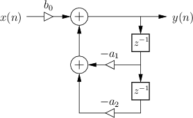
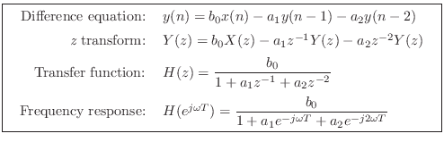
The signal flow graph for the general two-pole filter is given in Fig.B.5. We proceed as usual with the general analysis steps to obtain the following:
The numerator of ![]() is a constant, so there are no zeros other
than two at the origin of the
is a constant, so there are no zeros other
than two at the origin of the ![]() plane.
plane.
The coefficients ![]() and
and ![]() are called the denominator
coefficients, and they determine the two poles of
are called the denominator
coefficients, and they determine the two poles of ![]() .
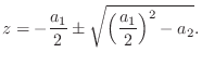
Using the quadratic formula, the poles are found to be located at
.
Using the quadratic formula, the poles are found to be located at
When both poles are real, the two-pole can be analyzed simply as a cascade of two one-pole sections, as in the previous section. That is, one can multiply pointwise two magnitude plots such as Fig.B.4a, and add pointwise two phase plots such as Fig.B.4b.
When the poles are complex, they can be written as
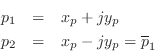
since they must form a complex-conjugate pair when ![]() and
and ![]() are real.
We may express them in polar form
as
are real.
We may express them in polar form
as
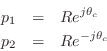
where
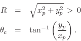
![]() is the pole radius, or distance from the origin in the
is the pole radius, or distance from the origin in the
![]() -plane. As discussed in Chapter 8, we must have
-plane. As discussed in Chapter 8, we must have ![]() for
stability of the two-pole filter. The angles
for
stability of the two-pole filter. The angles
![]() are the
poles' respective angles in the
are the
poles' respective angles in the ![]() plane. The pole angle
plane. The pole angle
![]() corresponds to the pole frequency
corresponds to the pole frequency ![]() via the
relation
via the
relation
If ![]() is sufficiently large (but less than 1 for stability), the
filter exhibits a resonanceB.2 at
radian frequency
is sufficiently large (but less than 1 for stability), the
filter exhibits a resonanceB.2 at
radian frequency
![]() . We may call
. We may call
![]() or
or ![]() the center frequency of the
resonator. Note, however, that the resonance frequency is not usually
the precise frequency of peak-gain in a two-pole resonator (see
Fig.B.9 on page
the center frequency of the
resonator. Note, however, that the resonance frequency is not usually
the precise frequency of peak-gain in a two-pole resonator (see
Fig.B.9 on page ![]() ).
The peak of the amplitude response is usually a little different
because each pole sits on the other's ``skirt,'' which is slanted.
(See §B.1.5 and §B.6 for an elaboration of this point.)
).
The peak of the amplitude response is usually a little different
because each pole sits on the other's ``skirt,'' which is slanted.
(See §B.1.5 and §B.6 for an elaboration of this point.)
Using polar form for the (complex) poles, the two-pole transfer
function can be expressed as
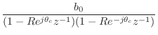
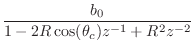
Comparing this to the transfer function derived from the difference equation, we may identify
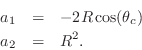
The difference equation can thus be rewritten as
Note that coefficient ![]() depends only on the pole radius R (which
determines damping) and is independent of the resonance frequency,
while
depends only on the pole radius R (which
determines damping) and is independent of the resonance frequency,
while ![]() is a function of both. As a result, we may retune
the resonance frequency of the two-pole filter section by modifying
is a function of both. As a result, we may retune
the resonance frequency of the two-pole filter section by modifying
![]() only.
only.
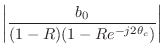
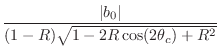
The gain at the resonant frequency
![]() , is found by
substituting
, is found by
substituting
![]() into
Eq.
into
Eq.![]() (B.1) to get
(B.1) to get
See §B.6 for details on how the resonance
gain (and peak gain) can be normalized as the tuning of ![]() is
varied in real time.
is
varied in real time.
Since the radius of both poles is ![]() , we must have
, we must have ![]() for filter
stability (§8.4). The
closer
for filter
stability (§8.4). The
closer ![]() is to 1, the higher the gain at the resonant frequency
is to 1, the higher the gain at the resonant frequency
![]() . If
. If ![]() , the filter degenerates to the form
, the filter degenerates to the form
![]() , which is a nothing but a scale factor. We can say that
when the two poles move to the origin of the
, which is a nothing but a scale factor. We can say that
when the two poles move to the origin of the ![]() plane, they are
canceled by the two zeros there.
plane, they are
canceled by the two zeros there.
Resonator Bandwidth in Terms of Pole Radius
The magnitude ![]() of a complex pole determines the
damping or bandwidth of the resonator. (Damping may be
defined as the reciprocal of the bandwidth.)
of a complex pole determines the
damping or bandwidth of the resonator. (Damping may be
defined as the reciprocal of the bandwidth.)
As derived in §8.5, when ![]() is close to 1, a reasonable
definition of 3dB-bandwidth
is close to 1, a reasonable
definition of 3dB-bandwidth ![]() is provided by
is provided by

where
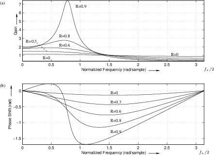
Figure B.6 shows a family of frequency responses for the
two-pole resonator obtained by setting ![]() and varying
and varying ![]() . The
value of
. The
value of ![]() in all cases is
in all cases is ![]() , corresponding to
, corresponding to
![]() . The analytic expressions for amplitude and phase response are
. The analytic expressions for amplitude and phase response are
![\begin{eqnarray*}
G(\omega)\! &=&
\!\frac{b_0}{\sqrt{[1 + a_1 \cos(\omega T) + a...
... + a_1 \cos(\omega T) + a_2 \cos(2\omega T)}\right]\qquad(b_0>0)
\end{eqnarray*}](http://www.dsprelated.com/josimages_new/filters/img1385.png)
where
![]() and
and ![]() .
.
 |
Next Section:
Two-Zero
Previous Section:
One-Pole


