


Pole-Zero Analysis
This chapter discusses pole-zero analysis of digital filters. Every digital filter can be specified by its poles and zeros (together with a gain factor). Poles and zeros give useful insights into a filter's response, and can be used as the basis for digital filter design. This chapter additionally presents the Durbin step-down recursion for checking filter stability by finding the reflection coefficients, including matlab code.
Going back to Eq.![]() (6.5), we can write the general transfer
function for the recursive LTI digital filter as
(6.5), we can write the general transfer
function for the recursive LTI digital filter as
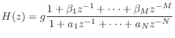
which is the same as Eq.
Assume, for simplicity, that none of the factors cancel out. The (possibly complex) numbers
The term ``pole'' makes sense when one plots the magnitude of ![]() as a
function of z. Since
as a
function of z. Since ![]() is complex, it may be taken to lie in a plane
(the
is complex, it may be taken to lie in a plane
(the ![]() plane). The magnitude of
plane). The magnitude of ![]() is real and therefore can be
represented by distance above the
is real and therefore can be
represented by distance above the ![]() plane. The plot appears as an
infinitely thin surface spanning in all directions over the
plane. The plot appears as an
infinitely thin surface spanning in all directions over the ![]() plane. The zeros are the points where the surface dips down to touch
the
plane. The zeros are the points where the surface dips down to touch
the ![]() plane. At high altitude, the poles look like thin, well,
``poles'' that go straight up forever, getting thinner the higher they
go.
plane. At high altitude, the poles look like thin, well,
``poles'' that go straight up forever, getting thinner the higher they
go.
Notice that the ![]() feedforward coefficients from the general
difference quation, Eq.
feedforward coefficients from the general
difference quation, Eq.![]() (5.1), give rise to
(5.1), give rise to ![]() zeros. Similarly,
the
zeros. Similarly,
the ![]() feedback coefficients in Eq.
feedback coefficients in Eq.![]() (5.1) give rise to
(5.1) give rise to ![]() poles.
Recall that we defined the filter order as the maximum of
poles.
Recall that we defined the filter order as the maximum of ![]() and
and ![]() in Eq.
in Eq.![]() (6.5). Therefore, the filter order equals the
number of poles or zeros, whichever is greater.
(6.5). Therefore, the filter order equals the
number of poles or zeros, whichever is greater.
Filter Order = Transfer Function Order
Recall that the
order of a polynomial
is defined as the highest
power of the polynomial variable. For example, the order of the
polynomial
![]() is 2. From Eq.
is 2. From Eq.![]() (8.1), we see that
(8.1), we see that ![]() is
the order of the transfer-function numerator polynomial in
is
the order of the transfer-function numerator polynomial in ![]() .
Similarly,
.
Similarly, ![]() is the order of the denominator polynomial in
is the order of the denominator polynomial in ![]() .
.
A rational function is any ratio of polynomials. That is,
![]() is a rational function if it can be written as
is a rational function if it can be written as

It turns out the transfer function can be viewed as a rational
function of either ![]() or
or ![]() without affecting order. Let
without affecting order. Let
![]() denote the order of a general LTI filter with transfer
function
denote the order of a general LTI filter with transfer
function ![]() expressible as in Eq.
expressible as in Eq.![]() (8.1). Then multiplying
(8.1). Then multiplying ![]() by
by ![]() gives a rational function of
gives a rational function of ![]() (as opposed to
(as opposed to ![]() )
that is also order
)
that is also order ![]() when viewed as a ratio of polynomials in
when viewed as a ratio of polynomials in ![]() .
Another way to reach this conclusion is to consider that replacing
.
Another way to reach this conclusion is to consider that replacing ![]() by
by ![]() is a conformal map [57] that inverts the
is a conformal map [57] that inverts the
![]() -plane with respect to the unit circle. Such a transformation
clearly preserves the number of poles and zeros, provided poles and
zeros at
-plane with respect to the unit circle. Such a transformation
clearly preserves the number of poles and zeros, provided poles and
zeros at ![]() and
and ![]() are either both counted or both not
counted.
are either both counted or both not
counted.
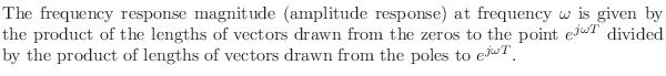
Graphical Computation of
Amplitude Response from
Poles and Zeros
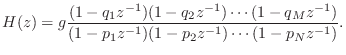
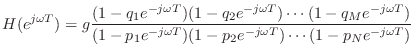
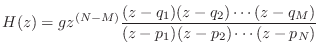
Now consider what happens when we take the factored form of the
general transfer function, Eq.![]() (8.2), and set
(8.2), and set ![]() to
to
![]() to get the frequency response in factored form:
to get the frequency response in factored form:
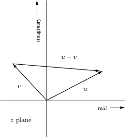
In the complex plane, the number
![]() is plotted at the
coordinates
is plotted at the
coordinates ![]() [84]. The difference of two vectors
[84]. The difference of two vectors
![]() and
and
![]() is
is
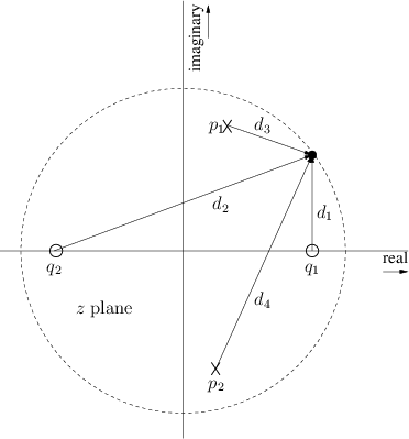
![]() , as shown in Fig.8.1. Translating the origin of the
vector
, as shown in Fig.8.1. Translating the origin of the
vector ![]() to the tip of
to the tip of ![]() shows that
shows that ![]() is an arrow drawn
from the tip of
is an arrow drawn
from the tip of ![]() to the tip of
to the tip of ![]() . The length of a vector is
unaffected by translation away from the origin. However, the angle of
a translated vector must be measured relative to a translated copy of
the real axis. Thus the term
. The length of a vector is
unaffected by translation away from the origin. However, the angle of
a translated vector must be measured relative to a translated copy of
the real axis. Thus the term
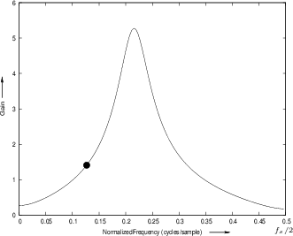
![]() may be drawn as an
arrow from the
may be drawn as an
arrow from the ![]() th zero to the point
th zero to the point
![]() on the unit
circle, and
on the unit
circle, and
![]() is an arrow from the
is an arrow from the ![]() th
pole. Therefore, each term in Eq.
th
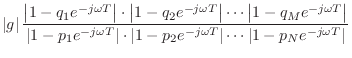
pole. Therefore, each term in Eq.![]() (8.3) is the length
of a vector drawn from a pole or zero to a single point on the unit
circle, as shown in Fig.8.2 for two poles and two zeros.
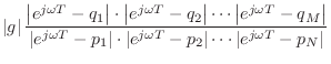
In summary:
(8.3) is the length
of a vector drawn from a pole or zero to a single point on the unit
circle, as shown in Fig.8.2 for two poles and two zeros.
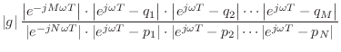
In summary:
 |
For example, the dc gain is obtained by multiplying the lengths of the
lines drawn from all poles and zeros to the point ![]() . The filter
gain at half the sampling rate is the product of the lengths of these
lines when drawn to the point
. The filter
gain at half the sampling rate is the product of the lengths of these
lines when drawn to the point ![]() . For an arbitrary frequency
. For an arbitrary frequency
![]() Hz, we draw arrows from the poles and zeros to the point
Hz, we draw arrows from the poles and zeros to the point
![]() . Thus, at the frequency where the arrows in
Fig.8.2 join, (which is slightly less than one-eighth the
sampling rate) the gain of this two-pole two-zero filter is
. Thus, at the frequency where the arrows in
Fig.8.2 join, (which is slightly less than one-eighth the
sampling rate) the gain of this two-pole two-zero filter is
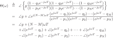
![]() . Figure 8.3 gives the complete amplitude
response for the poles and zeros shown in Fig.8.2. Before
looking at that, it is a good exercise to try sketching it by
inspection of the pole-zero diagram. It is usually easy to sketch a
qualitatively accurate amplitude-response directly from the poles and
zeros (to within a scale factor).
. Figure 8.3 gives the complete amplitude
response for the poles and zeros shown in Fig.8.2. Before
looking at that, it is a good exercise to try sketching it by
inspection of the pole-zero diagram. It is usually easy to sketch a
qualitatively accurate amplitude-response directly from the poles and
zeros (to within a scale factor).
 |
Graphical Phase Response Calculation
The phase response is almost as easy to evaluate graphically as is the amplitude response:
If ![]() is real, then
is real, then ![]() is either 0 or
is either 0 or ![]() . Terms of the
form
. Terms of the
form
![]() can be interpreted as a vector drawn from the point
can be interpreted as a vector drawn from the point ![]() to the point
to the point
![]() in the complex plane. The angle of
in the complex plane. The angle of
![]() is
the angle of the constructed vector (where a vector pointing
horizontally to the right has an angle of 0). Therefore, the phase
response at frequency
is
the angle of the constructed vector (where a vector pointing
horizontally to the right has an angle of 0). Therefore, the phase
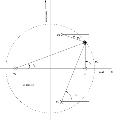
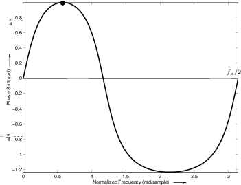
response at frequency ![]() Hz is again obtained by drawing lines from
all the poles and zeros to the point
Hz is again obtained by drawing lines from
all the poles and zeros to the point
![]() , as shown in
Fig.8.4. The angles of the lines from the zeros are added, and
the angles of the lines from the poles are subtracted. Thus, at the
frequency
, as shown in
Fig.8.4. The angles of the lines from the zeros are added, and
the angles of the lines from the poles are subtracted. Thus, at the
frequency ![]() the phase response of the two-pole two-zero filter
in the figure is
the phase response of the two-pole two-zero filter
in the figure is
![]() .
.
Note that an additional phase of
![]() radians appears when
the number of poles is not equal to the number of zeros. This factor
comes from writing the transfer function as
radians appears when
the number of poles is not equal to the number of zeros. This factor
comes from writing the transfer function as
 |
Stability Revisited
As defined earlier in §5.6 (page ![]() ), a
filter is said to be stable if its impulse response
), a
filter is said to be stable if its impulse response ![]() decays to 0 as
decays to 0 as ![]() goes to infinity.
In terms of poles and zeros, an irreducible filter transfer function
is stable if and only if all its poles are inside the unit circle in
the
goes to infinity.
In terms of poles and zeros, an irreducible filter transfer function
is stable if and only if all its poles are inside the unit circle in
the ![]() plane (as first discussed in §6.8.6). This is because
the transfer function is the z transform of the impulse response, and if
there is an observable (non-canceled) pole outside the unit circle,
then there is an exponentially increasing component of the impulse
response. To see this, consider a causal impulse response of the form
plane (as first discussed in §6.8.6). This is because
the transfer function is the z transform of the impulse response, and if
there is an observable (non-canceled) pole outside the unit circle,
then there is an exponentially increasing component of the impulse
response. To see this, consider a causal impulse response of the form
The signal
![]() has the z transform
has the z transform
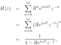
where the last step holds for
![]() , which is
true whenever
, which is
true whenever
![]() . Thus, the transfer function consists of a single pole at
. Thus, the transfer function consists of a single pole at
![]() , and it exists for
, and it exists for ![]() .9.1Now consider what happens when we let
.9.1Now consider what happens when we let ![]() become greater than 1. The
pole of
become greater than 1. The
pole of ![]() moves outside the unit circle, and the impulse response
has an exponentially increasing amplitude. (Note
moves outside the unit circle, and the impulse response
has an exponentially increasing amplitude. (Note
![]() .) Thus, the definition of stability is violated. Since the z transform
exists only for
.) Thus, the definition of stability is violated. Since the z transform
exists only for
![]() , we see that
, we see that ![]() implies that the
z transform no longer exists on the unit circle, so that the frequency
response becomes undefined!
implies that the
z transform no longer exists on the unit circle, so that the frequency
response becomes undefined!
The above one-pole analysis shows that a one-pole filter is stable if and only if its pole is inside the unit circle. In the case of an arbitrary transfer function, inspection of its partial fraction expansion (§6.8) shows that the behavior near any pole approaches that of a one-pole filter consisting of only that pole. Therefore, all poles must be inside the unit circle for stability.
In summary, we can state the following:
Isolated poles on the unit circle may be called marginally stable. The impulse response component corresponding to a single pole on the unit circle never decays, but neither does it grow.9.2 In physical modeling applications, marginally stable poles occur often in lossless systems, such as ideal vibrating string models [86].
Computing Reflection Coefficients to
Check Filter Stability
Since we know that a recursive filter is stable if and only if all its
poles have magnitude less than 1, an obvious method for checking
stability is to find the roots of the denominator polynomial ![]() in
the filter transfer function [Eq.
in
the filter transfer function [Eq.![]() (7.4)]. If the moduli of all roots
are less than 1, the filter is stable. This test works fine for
low-order filters (e.g., on the order of 100 poles or less), but it may
fail numerically at higher orders because the roots of a polynomial
are very sensitive to round-off error in the polynomial coefficients
[62]. It is therefore of interest to use a stability test
that is faster and more reliable numerically than polynomial
root-finding. Fortunately, such a test exists based on the filter
reflection coefficients.
(7.4)]. If the moduli of all roots
are less than 1, the filter is stable. This test works fine for
low-order filters (e.g., on the order of 100 poles or less), but it may
fail numerically at higher orders because the roots of a polynomial
are very sensitive to round-off error in the polynomial coefficients
[62]. It is therefore of interest to use a stability test
that is faster and more reliable numerically than polynomial
root-finding. Fortunately, such a test exists based on the filter
reflection coefficients.
It is a mathematical fact [48] that all poles of a recursive
filter are inside the unit circle if and only if all its reflection
coefficients (which are always real) are strictly between -1 and 1.
The full theory
associated with reflection coefficients is beyond the scope of this
book, but can be found in most modern treatments of
linear prediction [48,47] or speech
modeling [92,19,69]. An online
derivation appears in [86].9.3Here, we will settle for a simple recipe for computing the reflection
coefficients from the transfer-function denominator polynomial ![]() .
This recipe is called the step-down procedure,
Schur-Cohn stability test,
or Durbin recursion
[48], and it is essentially the same thing as the Schur
recursion (for allpass filters) or Levinson algorithm (for
autocorrelation functions of autoregressive stochastic processes)
[38].
.
This recipe is called the step-down procedure,
Schur-Cohn stability test,
or Durbin recursion
[48], and it is essentially the same thing as the Schur
recursion (for allpass filters) or Levinson algorithm (for
autocorrelation functions of autoregressive stochastic processes)
[38].
Step-Down Procedure
Let ![]() denote the
denote the ![]() th-order denominator polynomial of the
recursive filter transfer function
th-order denominator polynomial of the
recursive filter transfer function
![]() :
:
We have introduced the new subscript
In addition to the denominator polynomial ![]() , we need its
flip:
, we need its
flip:
The recursion begins by setting the
Otherwise, if
![]() , the polynomial order is decremented by 1
to yield
, the polynomial order is decremented by 1
to yield
![]() as follows (recall that
as follows (recall that ![]() is
monic):
is
monic):
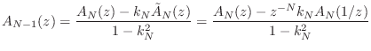
Next ![]() is set to
is set to
![]() , and the recursion continues
until
, and the recursion continues
until
![]() is reached, or
is reached, or
![]() is found for some
is found for some
![]() .
.
Whenever
![]() , the recursion halts prematurely, and the
filter is usually declared unstable (at best it is marginally
stable, meaning that it has at least one pole on the unit
circle).
, the recursion halts prematurely, and the
filter is usually declared unstable (at best it is marginally
stable, meaning that it has at least one pole on the unit
circle).
Note that the reflection coefficients can also be used to implement the digital filter in what are called lattice or ladder structures [48]. Lattice/ladder filters have superior numerical properties relative to direct-form filter structures based on the difference equation. As a result, they can be very important for fixed-point implementations such as in custom VLSI or low-cost (fixed-point) signal processing chips. Lattice/ladder structures are also a good point of departure for computational physical models of acoustic systems such as vibrating strings, wind instrument bores, and the human vocal tract [81,16,48].
Testing Filter Stability in Matlab
Figure 8.6 gives a listing of a matlab function stabilitycheck for testing the stability of a digital filter using the Durbin step-down recursion. Figure 8.7 lists a main program for testing stabilitycheck against the more prosaic method of factoring the transfer-function denominator and measuring the pole radii. The Durbin recursion is far faster than the method based on root-finding.
function [stable] = stabilitycheck(A);

N = length(A)-1; % Order of A(z)
stable = 1;      % stable unless shown otherwise
A = A(:);        % make sure it's a column vector
for i=N:-1:1
  rci=A(i+1);
  if abs(rci) >= 1
    stable=0;
    return;
  end
  A = (A(1:i) - rci * A(i+1:-1:2))/(1-rci^2);
% disp(sprintf('A[%d]=',i)); A(1:i)'
end
|
% TSC - test function stabilitycheck, comparing against
%       pole radius computation

N = 200; % polynomial order
M = 20; % number of random polynomials to generate
disp('Random polynomial test');
nunstp = 0; % count of unstable A polynomials
sctime = 0; % total time in stabilitycheck()
rftime = 0; % total time computing pole radii
for pol=1:M
  A = [1; rand(N,1)]'; % random polynomial
  tic;
  stable = stabilitycheck(A);
  et=toc;  % Typ. 0.02 sec Octave/Linux, 2.8GHz Pentium
  sctime = sctime + et;
  % Now do it the old fashioned way
  tic;
  poles = roots(A); % system poles
  pr = abs(poles);  % pole radii
  unst = (pr >= 1); % bit vector
  nunst = sum(unst);% number of unstable poles
  et=toc; % Typ. 2.9 sec Octave/Linux, 2.8GHz Pentium
  rftime = rftime + et;
  if stable, nunstp = nunstp + 1; end
  if (stable & nunst>0) | (~stable & nunst==0)
    error('*** stabilitycheck() and poles DISAGREE ***');
  end
end
disp(sprintf(...
     ['Out of %d random polynomials of order %d,',...
      ' %d were unstable'], M,N,nunstp));
|
When run in Octave over Linux 2.4 on a 2.8 GHz Pentium PC, the Durbin recursion is approximately 140 times faster than brute-force root-finding, as measured by the program listed in Fig.8.7.
Bandwidth of One Pole
A typical formula relating 3-dB bandwidth ![]() (in Hz) to the pole
radius
(in Hz) to the pole
radius ![]() is
is
where

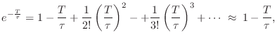
Time Constant of One Pole
A useful approximate formula giving the decay
time-constant9.4 ![]() (in
seconds) in terms of a pole radius
(in
seconds) in terms of a pole radius ![]() is
is

where
The exact relation between ![]() and
and ![]() is obtained by sampling an
exponential decay:
is obtained by sampling an
exponential decay:
Unstable Poles--Unit Circle Viewpoint
We saw in §8.4 that an LTI filter is stable if and only
if all of its poles are strictly inside the unit circle (![]() ) in
the complex
) in
the complex ![]() plane. In particular, a pole
plane. In particular, a pole ![]() outside the unit
circle (
outside the unit
circle (![]() ) gives rise to an impulse-response component
proportional to
) gives rise to an impulse-response component
proportional to ![]() which grows exponentially over time
which grows exponentially over time ![]() . We
also saw in §6.2 that the z transform of a growing exponential does
not not converge on the unit circle in the
. We
also saw in §6.2 that the z transform of a growing exponential does
not not converge on the unit circle in the ![]() plane. However, this
was the case for a causal exponential
plane. However, this
was the case for a causal exponential ![]() , where
, where ![]() is the unit-step function (which switches from 0 to 1 at time 0). If
the same exponential is instead anticausal, i.e., of the form
is the unit-step function (which switches from 0 to 1 at time 0). If
the same exponential is instead anticausal, i.e., of the form
![]() , then, as we'll see in this section, its z transform does exist on
the unit circle, and the pole is in exactly the same place as in the
causal case. Therefore,to unambiguously invert a z transform, we must know
its region of convergence. The critical question is whether
the region of convergence includes the unit circle: If it does, then
each pole outside the unit circle corresponds to an anticausal, finite
energy, exponential, while each pole inside corresponds to the usual
causal decaying exponential.
, then, as we'll see in this section, its z transform does exist on
the unit circle, and the pole is in exactly the same place as in the
causal case. Therefore,to unambiguously invert a z transform, we must know
its region of convergence. The critical question is whether
the region of convergence includes the unit circle: If it does, then
each pole outside the unit circle corresponds to an anticausal, finite
energy, exponential, while each pole inside corresponds to the usual
causal decaying exponential.
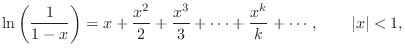
Geometric Series
The essence of the situation can be illustrated using a simple
geometric series. Let ![]() be any real (or complex) number. Then we
have
be any real (or complex) number. Then we
have
![$\displaystyle \frac{1}{1-R} \eqsp \frac{-R^{-1}}{1-R^{-1}}
\eqsp -R^{-1}\left[1 + R^{-1} + R^{-2} + R^{-3} + \cdots \right]
$](http://www.dsprelated.com/josimages_new/filters/img1083.png)
One-Pole Transfer Functions
We can apply the same analysis to a one-pole transfer function.
Let
![]() denote any real or complex number:
denote any real or complex number:
Now consider the rewritten case:
![\begin{eqnarray*}
\frac{1}{1-pz^{-1}} &=& \frac{-p^{-1}z}{1-p^{-1}z} \\
&=& -p^...
...cdots\right]\\
&\leftrightarrow& - u(-n-1)p^n,\quad n\in{\bf Z}
\end{eqnarray*}](http://www.dsprelated.com/josimages_new/filters/img1092.png)
where the inverse z transform is the inverse bilateral z transform. In this
case, the convergence criterion is
![]() , or
, or ![]() , and
this region includes the unit circle when
, and
this region includes the unit circle when ![]() .
.
In summary, when the region-of-convergence of the z transform is assumed to
include the unit circle of the ![]() plane, poles inside the unit circle
correspond to stable, causal, decaying exponentials, while poles
outside the unit circle correspond to anticausal exponentials that
decay toward time
plane, poles inside the unit circle
correspond to stable, causal, decaying exponentials, while poles
outside the unit circle correspond to anticausal exponentials that
decay toward time ![]() , and stop before time zero.
, and stop before time zero.
Figure 8.8 illustrates the two types of exponentials (causal and anticausal) that correspond to poles (inside and outside the unit circle) when the z transform region of convergence is defined to include the unit circle.
myFourFiguresToWidthpolesout11polesout21polesout12polesout220.52Left column:
Causal exponential decay, pole at ![]() . Right column: Anticausal
exponential decay, pole at
. Right column: Anticausal
exponential decay, pole at ![]() . Top: Pole-zero diagram.
Bottom: Corresponding impulse response, assuming the region of
convergence includes the unit circle in the
. Top: Pole-zero diagram.
Bottom: Corresponding impulse response, assuming the region of
convergence includes the unit circle in the ![]() plane.
plane.
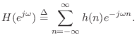
Poles and Zeros of the Cepstrum
The complex cepstrum of a sequence ![]() is typically defined
as the inverse Fourier transform of its log spectrum
[60]
is typically defined
as the inverse Fourier transform of its log spectrum
[60]
![$\displaystyle {\tilde h}(n)\isdef \frac{1}{2\pi}\int_{-\pi}^\pi \ln[H(e^{j\omega})] e^{j\omega n}d\omega,
$](http://www.dsprelated.com/josimages_new/filters/img1095.png)
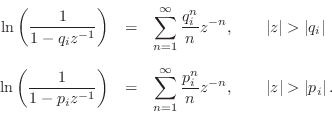
From Eq.![]() (8.2), the log z transform can be written in terms of the
factored form as
(8.2), the log z transform can be written in terms of the
factored form as
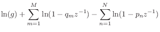
where
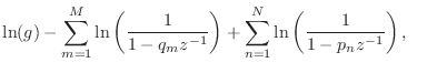
Since the region of convergence of the z transform must include the unit
circle (where the spectrum (DTFT) is defined), we see that the
Maclaurin expansion gives us the inverse z transform of all terms of
Eq.![]() (8.9) corresponding to poles and zeros inside the unit
circle of the
(8.9) corresponding to poles and zeros inside the unit
circle of the ![]() plane. Since the poles must be inside the unit
circle anyway for stability, this restriction is normally not binding
for the poles. However, zeros outside the unit circle--so-called
``non-minimum-phase zeros''--are used quite often in practice.
plane. Since the poles must be inside the unit
circle anyway for stability, this restriction is normally not binding
for the poles. However, zeros outside the unit circle--so-called
``non-minimum-phase zeros''--are used quite often in practice.
For a zero (or pole) outside the unit circle, we may rewrite the
corresponding term of Eq.![]() (8.9) as
(8.9) as
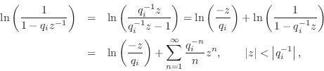
where we used the Maclaurin series expansion for
![]() once
again with the region of convergence including the unit circle. The
infinite sum in this expansion is now the bilateral z transform of an
anticausal sequence, as discussed in §8.7. That is,
the time-domain sequence is zero for nonnegative times (
once
again with the region of convergence including the unit circle. The
infinite sum in this expansion is now the bilateral z transform of an
anticausal sequence, as discussed in §8.7. That is,
the time-domain sequence is zero for nonnegative times (![]() ) and
the sequence decays in the direction of time minus-infinity. The
factored-out terms
) and
the sequence decays in the direction of time minus-infinity. The
factored-out terms ![]() and
and ![]() , for all poles and zeros
outside the unit circle, can be collected together and associated with
the overall gain factor
, for all poles and zeros
outside the unit circle, can be collected together and associated with
the overall gain factor ![]() in Eq.
in Eq.![]() (8.9), resulting in a modified
scaling and time-shift for the original sequence
(8.9), resulting in a modified
scaling and time-shift for the original sequence ![]() which can be
dealt with separately [60].
which can be
dealt with separately [60].
When all poles and zeros are inside the unit circle, the complex cepstrum is causal and can be expressed simply in terms of the filter poles and zeros as
![$\displaystyle {\tilde h}(n) = \left\{\begin{array}{ll}
\ln(g), & n=0 \\ [5pt]
\...
...ystyle\sum_{k=1}^M \frac{q_k^n}{n}, & n=1,2,3,\ldots\,, \\
\end{array}\right.
$](http://www.dsprelated.com/josimages_new/filters/img1115.png)
In summary, each stable pole contributes a positive decaying
exponential (weighted by ![]() ) to the complex cepstrum, while each
zero inside the unit circle contributes a negative
weighted-exponential of the same type. The decaying exponentials
start at time 1 and have unit amplitude (ignoring the
) to the complex cepstrum, while each
zero inside the unit circle contributes a negative
weighted-exponential of the same type. The decaying exponentials
start at time 1 and have unit amplitude (ignoring the ![]() weighting)
in the sense that extrapolating them to time 0 (without the
weighting)
in the sense that extrapolating them to time 0 (without the ![]() weighting) would use the values
weighting) would use the values ![]() and
and
![]() . The
decay rates are faster when the poles and zeros are well inside the
unit circle, but cannot decay slower than
. The
decay rates are faster when the poles and zeros are well inside the
unit circle, but cannot decay slower than ![]() .
.
On the other hand, poles and zeros outside the unit circle contribute anticausal exponentials to the complex cepstrum, negative for the poles and positive for the zeros.
Conversion to Minimum Phase
As discussed in §11.7, any spectrum can be converted to minimum-phase form (without affecting the spectral magnitude) by computing its cepstrum and replacing any anticausal components with corresponding causal components. In other words, the anticausal part of the cepstrum, if any, is ``flipped'' about time zero so that it adds to the causal part. Doing this corresponds to reflecting non-minimum phase zeros (and any unstable poles) inside the unit circle in a manner that preserves spectral magnitude. The original spectral phase is then replaced by the unique minimum phase corresponding to the given spectral magnitude.
A matlab listing for computing a minimum-phase spectrum from the magnitude spectrum is given in §J.11.
Hilbert Transform Relations
Closely related to the cepstrum are the so-called Hilbert transform relations that relate the real and imaginary parts of the spectra of causal signals. In particular, for minimum-phase spectra, the cepstrum is causal, and this means that the log-magnitude and phase form a Hilbert-transform pair. Methods for designing allpass filters have been based on this relationship (see §B.2.2). For more about cepstra and Hilbert transform relations, see [60].
Pole-Zero Analysis Problems
See http://ccrma.stanford.edu/~jos/filtersp/Pole_Zero_Analysis_Problems.html.
Next Section:
Implementation Structures for Recursive Digital Filters
Previous Section:
Frequency Response Analysis


