


Single-Reed Theory
![\includegraphics[scale=0.9]{eps/fReedSchematic}](http://www.dsprelated.com/josimages_new/pasp/img2321.png)
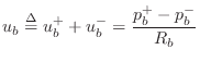
A simplified diagram of the clarinet mouthpiece is shown in
Fig. 9.40. The pressure in the mouth is assumed
to be a constant value ![]() , and the bore pressure
, and the bore pressure ![]() is defined
located at the mouthpiece. Any pressure drop
is defined
located at the mouthpiece. Any pressure drop
![]() across
the mouthpiece causes a flow
across
the mouthpiece causes a flow ![]() into the mouthpiece through the
reed-aperture impedance
into the mouthpiece through the
reed-aperture impedance
![]() which changes as a function of
which changes as a function of
![]() since the reed position is affected by
since the reed position is affected by
![]() . To a first
approximation, the clarinet reed can be regarded as a spring flap
regulated Bernoulli flow (§B.7.5), [249]).
This model has been verified well experimentally until the reed is
about to close, at which point viscosity effects begin to appear
[102]. It has also been verified that the mass
of the reed can be neglected to first order,10.18 so that
. To a first
approximation, the clarinet reed can be regarded as a spring flap
regulated Bernoulli flow (§B.7.5), [249]).
This model has been verified well experimentally until the reed is
about to close, at which point viscosity effects begin to appear
[102]. It has also been verified that the mass
of the reed can be neglected to first order,10.18 so that
![]() is a
positive real number for all values of
is a
positive real number for all values of
![]() . Possibly the most
important neglected phenomenon in this model is sound generation due
to turbulence of the flow, especially near reed closure. Practical
synthesis models have always included a noise component of some sort
which is modulated by the reed [431], despite a lack of firm
basis in acoustic measurements to date.
. Possibly the most
important neglected phenomenon in this model is sound generation due
to turbulence of the flow, especially near reed closure. Practical
synthesis models have always included a noise component of some sort
which is modulated by the reed [431], despite a lack of firm
basis in acoustic measurements to date.
The fundamental equation governing the action of the reed is continuity of volume velocity, i.e.,
where
and
is the volume velocity corresponding to the incoming pressure wave
In operation, the mouth pressure ![]() and incoming traveling bore pressure
and incoming traveling bore pressure
![]() are given, and the reed computation must produce an outgoing bore
pressure
are given, and the reed computation must produce an outgoing bore
pressure ![]() which satisfies (9.35), i.e., such that
which satisfies (9.35), i.e., such that
Solving for
It is helpful to normalize (9.38) as follows: Define
![]() , and note that
, and note that
![]() , where
, where
![]() . Then (9.38) can be multiplied through by
. Then (9.38) can be multiplied through by ![]() and
written as
and
written as
![]() , or
, or
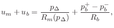
The solution is obtained by plotting
| (10.40) |
An example of the qualitative appearance of ![]() overlaying
overlaying
![]() is shown in Fig. 9.41.
is shown in Fig. 9.41.
![\includegraphics[width=\twidth]{eps/fReedRelations}](http://www.dsprelated.com/josimages_new/pasp/img2346.png)
Scattering-Theoretic Formulation
Equation (9.38) can be solved for ![]() to obtain
to obtain

where
 |
(10.44) |
We interpret
Since the mouthpiece of a clarinet is nearly closed,
![]() which
implies
which
implies
![]() and
and
![]() . In the limit as
. In the limit as ![]() goes to
infinity relative to
goes to
infinity relative to ![]() , (9.42) reduces to the simple form of a
rigidly capped acoustic tube, i.e.,
, (9.42) reduces to the simple form of a
rigidly capped acoustic tube, i.e.,
![]() .
If it were possible to open the reed wide enough to achieve
matched impedance,
.
If it were possible to open the reed wide enough to achieve
matched impedance, ![]() , then we would have
, then we would have ![]() and
and ![]() , in
which case
, in
which case
![]() , with no reflection of
, with no reflection of ![]() , as expected. If
the mouthpiece is removed altogether to give
, as expected. If
the mouthpiece is removed altogether to give ![]() (regarding it now as a
tube section of infinite radius), then
(regarding it now as a
tube section of infinite radius), then ![]() ,
, ![]() , and
, and
![]() .
.
Computational Methods
Since finding the intersection of ![]() and
and
![]() requires an expensive
iterative algorithm with variable convergence times, it is not well suited
for real-time operation. In this section, fast algorithms based on
precomputed nonlinearities are described.
requires an expensive
iterative algorithm with variable convergence times, it is not well suited
for real-time operation. In this section, fast algorithms based on
precomputed nonlinearities are described.
Let ![]() denote half-pressure
denote half-pressure ![]() , i.e.,
, i.e.,
![]() and
and
![]() . Then (9.43) becomes
. Then (9.43) becomes
Subtracting this equation from
The last expression above can be used to precompute
| (10.47) |
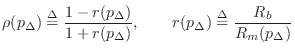
(9.45) becomes
This is the form chosen for implementation in Fig. 9.39 [431]. The control variable is mouth half-pressure
Because the table contains a coefficient rather than a signal value, it
can be more heavily quantized both in address space and word length than
a direct lookup of a signal value such as
![]() or the like. A
direct signal lookup, though requiring much higher resolution, would
eliminate the multiplication associated with the scattering coefficient.
For example, if
or the like. A
direct signal lookup, though requiring much higher resolution, would
eliminate the multiplication associated with the scattering coefficient.
For example, if ![]() and
and ![]() are 16-bit signal samples,
the table would contain on the order of 64K 16-bit
are 16-bit signal samples,
the table would contain on the order of 64K 16-bit
![]() samples.
Clearly, some compression of this table would be desirable. Since
samples.
Clearly, some compression of this table would be desirable. Since
![]() is smoothly varying, significant compression is in fact
possible. However, because the table is directly in the signal path,
comparatively little compression can be done while maintaining full
audio quality (such as 16-bit accuracy).
is smoothly varying, significant compression is in fact
possible. However, because the table is directly in the signal path,
comparatively little compression can be done while maintaining full
audio quality (such as 16-bit accuracy).
![\includegraphics[width=4in]{eps/fReedTable}](http://www.dsprelated.com/josimages_new/pasp/img2382.png)
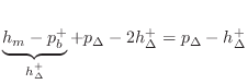
In the field of computer music, it is customary to use simple piecewise linear functions for functions other than signals at the audio sampling rate, e.g., for amplitude envelopes, FM-index functions, and so on [382,380]. Along these lines, good initial results were obtained [431] using the simplified qualitatively chosen reed table
depicted in Fig. 9.42 for
Another variation is to replace the table-lookup contents by a piecewise polynomial approximation. While less general, good results have been obtained in practice [89,91,92]. For example, one of the SynthBuilder [353] clarinet patches employs this technique using a cubic polynomial.
An intermediate approach between table lookups and polynomial approximations is to use interpolated table lookups. Typically, linear interpolation is used, but higher order polynomial interpolation can also be considered (see Chapter 4).
Clarinet Synthesis Implementation Details
To finish off the clarinet example, the remaining details of the SynthBuilder clarinet patch Clarinet2.sb are described.
The input mouth pressure is summed with a small amount of white noise,
corresponding to turbulence. For example, 0.1% is generally used as a
minimum, and larger amounts are appropriate during the attack of a note.
Ideally, the turbulence level should be computed automatically as a
function of pressure drop
![]() and reed opening geometry
[141,530]. It should also be lowpass filtered
as predicted by theory.
and reed opening geometry
[141,530]. It should also be lowpass filtered
as predicted by theory.
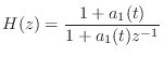
Referring to Fig. 9.39, the reflection filter is a simple one-pole with transfer function
 |
(10.50) |
where
Legato note transitions are managed using two delay line taps and cross-fading from one to the other during a transition [208,441,405]. In general, legato problems arise when the bore length is changed suddenly while sounding, corresponding to a new fingering. The reason is that really the model itself should be changed during a fingering change from that of a statically terminated bore to that of a bore with a new scattering junction appearing where each ``finger'' is lifting, and with disappearing scattering junctions where tone holes are being covered. In addition, if a hole is covered abruptly (especially when there are large mechanical caps, as in the saxophone), there will also be new signal energy injected in both directions on the bore in superposition with the signal scattering. As a result of this ideal picture, is difficult to get high quality legato performance using only a single delay line.
A reduced-cost, approximate solution for obtaining good sounding note transitions in a single delay-line model was proposed in [208]. In this technique, the bore delay line is ``branched'' during the transition, i.e., a second feedback loop is formed at the new loop delay, thus forming two delay lines sharing the same memory, one corresponding to the old pitch and the other corresponding to the new pitch. A cross-fade from the old-pitch delay to the new-pitch delay sounds good if the cross-fade time and duration are carefully chosen. Another way to look at this algorithm is in terms of ``read pointers'' and ``write pointers.'' A normal delay line consists of a single write pointer followed by a single read pointer, delayed by one period. During a legato transition, we simply cross-fade from a read-pointer at the old-pitch delay to a read-pointer at the new-pitch delay. In this type of implementation, the write-pointer always traverses the full delay memory corresponding to the minimum supported pitch in order that read-pointers may be instantiated at any pitch-period delay at any time. Conceptually, this simplified model of note transitions can be derived from the more rigorous model by replacing the tone-hole scattering junction by a single reflection coefficient.
STK software implementing a model as in Fig.9.39 can be found in the file Clarinet.cpp.
Next Section:
Tonehole Modeling
Previous Section:
A View of Single-Reed Oscillation


