


Delay-Line and Signal Interpolation
It is often necessary for a delay line to vary in length. Consider, for example, simulating a sound ray as in Fig.2.8 when either the source or listener is moving. In this case, separate read and write pointers are normally used (as opposed to a shared read-write pointer in Fig.2.2). Additionally, for good quality audio, it is usually necessary to interpolate the delay-line length rather than ``jumping'' between integer numbers of samples. This is typically accomplished using an interpolating read, but interpolating writes are also used (e.g., for true Doppler simulation, as described in §5.9).
Delay-Line Interpolation
As mentioned above, when an audio delay line needs to vary smoothly over time, some form of interpolation between samples is usually required to avoid ``zipper noise'' in the output signal as the delay length changes. There is a hefty literature on ``fractional delay'' in discrete-time systems, and the survey in [267] is highly recommended.
This section will describe the most commonly used cases. Linear interpolation is perhaps most commonly used because it is very straightforward and inexpensive, and because it sounds very good when the signal bandwidth is small compared with half the sampling rate. For a delay line in a nearly lossless feedback loop, such as in a vibrating string simulation, allpass interpolation is sometimes a better choice since it costs the same as linear interpolation in the first-order case and has no gain distortion. (Feedback loops can be very sensitive to gain distortions.) Finally, in later sections, some higher-order interpolation methods are described.
Linear Interpolation
Linear interpolation works by effectively drawing a straight line between two neighboring samples and returning the appropriate point along that line.
More specifically, let ![]() be a number between 0 and 1 which
represents how far we want to interpolate a signal
be a number between 0 and 1 which
represents how far we want to interpolate a signal ![]() between time
between time
![]() and time
and time ![]() . Then we can define the linearly interpolated
value
. Then we can define the linearly interpolated
value
![]() as follows:
as follows:
For
One-Multiply Linear Interpolation
Note that by factoring out ![]() , we can obtain a one-multiply
form,
, we can obtain a one-multiply
form,
Fractional Delay Filtering by Linear Interpolation
![\includegraphics[width=\twidth]{eps/delayli}](http://www.dsprelated.com/josimages_new/pasp/img934.png)
A linearly interpolated delay line is depicted in Fig.4.1. In
contrast to Eq.![]() (4.1), we interpolate linearly between times
(4.1), we interpolate linearly between times
![]() and
and ![]() , and
, and ![]() is called the fractional delay in
samples. The first-order (linear-interpolating) filter following the
delay line in Fig.4.1 may be called a fractional delay
filter [267]. Equation (4.1), on the other hand, expresses the more
general case of an interpolated table lookup, where
is called the fractional delay in
samples. The first-order (linear-interpolating) filter following the
delay line in Fig.4.1 may be called a fractional delay
filter [267]. Equation (4.1), on the other hand, expresses the more
general case of an interpolated table lookup, where ![]() is
regarded as a table of samples and
is
regarded as a table of samples and
![]() is regarded as an
interpolated table-lookup based on the samples stored at indices
is regarded as an
interpolated table-lookup based on the samples stored at indices ![]() and
and ![]() .
.
The difference between a fractional delay filter and an interpolated table lookup is that table-lookups can ``jump around,'' while fractional delay filters receive a sequential stream of input samples and produce a corresponding sequential stream of interpolated output values. As a result of this sequential access, fractional delay filters may be recursive IIR digital filters (provided the desired delay does not change too rapidly over time). In contrast, ``random-access'' interpolated table lookups are typically implemented using weighted linear combinations, making them equivalent to nonrecursive FIR filters in the sequential case.5.1
The C++ class implementing a linearly interpolated delay line in the Synthesis Tool Kit (STK) is called DelayL.
The frequency response of linear interpolation for fixed fractional
delay (![]() fixed in Fig.4.1) is shown in Fig.4.2.
From inspection of Fig.4.1, we see that linear interpolation is
a one-zero FIR filter. When used to provide a fixed fractional delay,
the filter is linear and time-invariant (LTI). When the fractional delay
fixed in Fig.4.1) is shown in Fig.4.2.
From inspection of Fig.4.1, we see that linear interpolation is
a one-zero FIR filter. When used to provide a fixed fractional delay,
the filter is linear and time-invariant (LTI). When the fractional delay ![]() changes over time, it is a linear time-varying filter.
changes over time, it is a linear time-varying filter.
![\includegraphics[width=\twidth]{eps/linear1}](http://www.dsprelated.com/josimages_new/pasp/img937.png) |
Linear interpolation sounds best when the signal is oversampled. Since natural audio spectra tend to be relatively concentrated at low frequencies, linear interpolation tends to sound very good at high sampling rates.
When interpolation occurs inside a feedback loop, such as in digital waveguide models for vibrating strings (see Chapter 6), errors in the amplitude response can be highly audible (particularly when the loop gain is close to 1, as it is for steel strings, for example). In these cases, it is possible to eliminate amplitude error (at some cost in delay error) by using an allpass filter for delay-line interpolation.
First-Order Allpass Interpolation
A delay line interpolated by a first-order allpass filter is drawn in Fig.4.3.
![\includegraphics[width=\twidth]{eps/delayai}](http://www.dsprelated.com/josimages_new/pasp/img938.png)
Intuitively, ramping the coefficients of the allpass gradually ``grows'' or ``hides'' one sample of delay. This tells us how to handle resets when crossing sample boundaries.
The difference equation is
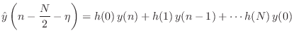
![\begin{eqnarray*}
{\hat x}(n-\Delta) \isdef y(n) &=& \eta \cdot x(n) + x(n-1) - ...
...y(n-1) \\
&=& \eta \cdot \left[ x(n) - y(n-1)\right] + x(n-1).
\end{eqnarray*}](http://www.dsprelated.com/josimages_new/pasp/img939.png)
Thus, like linear interpolation, first-order allpass interpolation requires only one multiply and two adds per sample of output.
The transfer function is
At low frequencies (
Figure 4.4 shows the phase delay of the first-order digital allpass filter for a variety of desired delays at dc. Since the amplitude response of any allpass is 1 at all frequencies, there is no need to plot it.
![\includegraphics[width=\twidth]{eps/allpass1}](http://www.dsprelated.com/josimages_new/pasp/img943.png)
The first-order allpass interpolator is generally controlled by
setting its dc delay to the desired delay. Thus, for a given desired
delay ![]() , the allpass coefficient is (from
Eq.
, the allpass coefficient is (from
Eq.![]() (4.3))
(4.3))

Note that, unlike linear interpolation, allpass interpolation is not suitable for ``random access'' interpolation in which interpolated values may be requested at any arbitrary time in isolation. This is because the allpass is recursive so that it must run for enough samples to reach steady state. However, when the impulse response is reasonably short, as it is for delays near one sample, it can in fact be used in ``random access mode'' by giving it enough samples with which to work.
![\includegraphics[width=4.8in]{eps/ap1pz}](http://www.dsprelated.com/josimages_new/pasp/img949.png)
The STK class implementing allpass-interpolated delay is DelayA.
Minimizing First-Order Allpass Transient Response
In addition to approaching a pole-zero cancellation at ![]() , another
undesirable artifact appears as
, another
undesirable artifact appears as
![]() : The transient
response also becomes long when the pole at
: The transient
response also becomes long when the pole at ![]() gets close to
the unit circle.
gets close to
the unit circle.
A plot of the impulse response for
![]() is shown in
Fig.4.6. We see a lot of ``ringing'' near half the sampling rate.
We actually should expect this from the nonlinear-phase
distortion which is clearly evident near half the sampling rate in
Fig.4.4. We can interpret this phenomenon as the signal
components near half the sampling rate being delayed by different
amounts than other frequencies, therefore ``sliding out of alignment''
with them.
is shown in
Fig.4.6. We see a lot of ``ringing'' near half the sampling rate.
We actually should expect this from the nonlinear-phase
distortion which is clearly evident near half the sampling rate in
Fig.4.4. We can interpret this phenomenon as the signal
components near half the sampling rate being delayed by different
amounts than other frequencies, therefore ``sliding out of alignment''
with them.
![\includegraphics[width=\twidth]{eps/ap1ir}](http://www.dsprelated.com/josimages_new/pasp/img952.png)
For audio applications, we would like to keep the impulse-response
duration short enough to sound ``instantaneous.'' That is, we do not
wish to have audible ``ringing'' in the time domain near ![]() . For
high quality sampling rates, such as larger than
. For
high quality sampling rates, such as larger than ![]() kHz, there
is no issue of direct audibility, since the ringing is above the range
of human hearing. However, it is often convenient, especially for
research prototyping, to work at lower sampling rates where
kHz, there
is no issue of direct audibility, since the ringing is above the range
of human hearing. However, it is often convenient, especially for
research prototyping, to work at lower sampling rates where ![]() is
audible. Also, many commercial products use such sampling rates to
save costs.
is
audible. Also, many commercial products use such sampling rates to
save costs.
Since the time constant of decay, in samples, of the impulse response
of a pole of radius ![]() is approximately
is approximately
For example, suppose 100 ms is chosen as the maximum ![]() allowed
at a sampling rate of
allowed
at a sampling rate of
![]() . Then applying the above constraints
yields
. Then applying the above constraints
yields
![]() , corresponding to the allowed delay range
, corresponding to the allowed delay range
![]() .
.
Linear Interpolation as Resampling
Convolution Interpretation
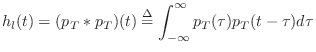
Linearly interpolated fractional delay is equivalent to filtering and resampling a weighted impulse train (the input signal samples) with a continuous-time filter having the simple triangular impulse response
![$\displaystyle h_l(t) = \left\{\begin{array}{ll} 1-\left\vert t/T\right\vert, & ...
...ght\vert\leq T, \\ [5pt] 0, & \hbox{otherwise}. \\ \end{array} \right. \protect$](http://www.dsprelated.com/josimages_new/pasp/img959.png)
Convolution of the weighted impulse train with
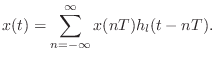
This continuous result can then be resampled at the desired fractional delay.
In discrete time processing, the operation Eq.![]() (4.5) can be
approximated arbitrarily closely by digital upsampling by a
large integer factor
(4.5) can be
approximated arbitrarily closely by digital upsampling by a
large integer factor ![]() , delaying by
, delaying by ![]() samples (an integer), then
finally downsampling by
samples (an integer), then
finally downsampling by ![]() , as depicted in Fig.4.7
[96]. The integers
, as depicted in Fig.4.7
[96]. The integers ![]() and
and ![]() are chosen so that
are chosen so that
![]() , where
, where ![]() the desired fractional delay.
the desired fractional delay.
![\includegraphics[width=0.8\twidth]{eps/polyphaseli}](http://www.dsprelated.com/josimages_new/pasp/img963.png)
The convolution interpretation of linear interpolation, Lagrange interpolation, and others, is discussed in [407].
Frequency Response of Linear Interpolation
Since linear interpolation can be expressed as a convolution of the
samples with a triangular pulse, we can derive the frequency
response of linear interpolation. Figure 4.7 indicates that
the triangular pulse ![]() serves as an anti-aliasing lowpass
filter for the subsequent downsampling by
serves as an anti-aliasing lowpass
filter for the subsequent downsampling by ![]() . Therefore, it should
ideally ``cut off'' all frequencies higher than
. Therefore, it should
ideally ``cut off'' all frequencies higher than ![]() .
.
Triangular Pulse as Convolution of Two Rectangular Pulses
The 2-sample wide triangular pulse ![]() (Eq.
(Eq.![]() (4.4)) can be
expressed as a convolution of the one-sample rectangular pulse with
itself.
(4.4)) can be
expressed as a convolution of the one-sample rectangular pulse with
itself.
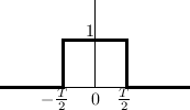
The one-sample rectangular pulse is shown in Fig.4.8 and may be defined analytically as
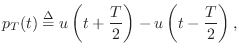
![$\displaystyle u(t) \isdef \left\{\begin{array}{ll}
1, & t\geq 0 \\ [5pt]
0, & t<0 \\
\end{array}\right..
$](http://www.dsprelated.com/josimages_new/pasp/img968.png)
Linear Interpolation Frequency Response
Since linear interpolation is a convolution of the samples with a
triangular pulse
![]() (from Eq.
(from Eq.![]() (4.5)),
the frequency response of the interpolation is given by the Fourier
transform
(4.5)),
the frequency response of the interpolation is given by the Fourier
transform ![]() , which yields a
sinc
, which yields a
sinc![]() function. This frequency
response applies to linear interpolation from discrete time to
continuous time. If the output of the interpolator is also sampled,
this can be modeled by sampling the continuous-time interpolation
result in Eq.
function. This frequency
response applies to linear interpolation from discrete time to
continuous time. If the output of the interpolator is also sampled,
this can be modeled by sampling the continuous-time interpolation
result in Eq.![]() (4.5), thereby aliasing the
sinc
(4.5), thereby aliasing the
sinc![]() frequency
response, as shown in Fig.4.9.
frequency
response, as shown in Fig.4.9.
![\includegraphics[width=3in]{eps/sincsquared}](http://www.dsprelated.com/josimages_new/pasp/img979.png)
In slightly more detail, from
![]() , and
, and
![]() sinc
sinc![]() , we have
, we have
The Fourier transform of ![]() is the same function aliased on
a block of size
is the same function aliased on
a block of size ![]() Hz. Both
Hz. Both ![]() and its alias are plotted
in Fig.4.9. The example in this figure pertains to an
output sampling rate which is
and its alias are plotted
in Fig.4.9. The example in this figure pertains to an
output sampling rate which is ![]() times that of the input signal.
In other words, the input signal is upsampled by a factor of
times that of the input signal.
In other words, the input signal is upsampled by a factor of ![]() using linear interpolation. The ``main lobe'' of the interpolation
frequency response
using linear interpolation. The ``main lobe'' of the interpolation
frequency response ![]() contains the original signal bandwidth;
note how it is attenuated near half the original sampling rate (
contains the original signal bandwidth;
note how it is attenuated near half the original sampling rate (![]() in Fig.4.9). The ``sidelobes'' of the frequency response
contain attenuated copies of the original signal bandwidth (see
the DFT stretch theorem), and thus constitute spectral imaging
distortion in the final output (sometimes also referred to as a kind
of ``aliasing,'' but, for clarity, that term will not be used for
imaging distortion in this book). We see that the frequency response
of linear interpolation is less than ideal in two ways:
in Fig.4.9). The ``sidelobes'' of the frequency response
contain attenuated copies of the original signal bandwidth (see
the DFT stretch theorem), and thus constitute spectral imaging
distortion in the final output (sometimes also referred to as a kind
of ``aliasing,'' but, for clarity, that term will not be used for
imaging distortion in this book). We see that the frequency response
of linear interpolation is less than ideal in two ways:
- The spectrum is ``rolled'' off near half the sampling rate. In fact, it is nowhere flat within the ``passband'' (-1 to 1 in Fig.4.9).
- Spectral imaging distortion is suppressed by only 26 dB (the level of the first sidelobe in Fig.4.9.
Special Cases
In the limiting case of ![]() , the input and output sampling rates are
equal, and all sidelobes of the frequency response
, the input and output sampling rates are
equal, and all sidelobes of the frequency response ![]() (partially
shown in Fig.4.9) alias into the main lobe.
(partially
shown in Fig.4.9) alias into the main lobe.
If the output is sampled at the same exact time instants as the input
signal, the input and output are identical. In terms of the aliasing
picture of the previous section, the frequency response aliases to a
perfect flat response over
![]() , with all spectral images
combining coherently under the flat gain. It is important in this
reconstruction that, while the frequency response of the underlying
continuous interpolating filter is aliased by sampling, the signal
spectrum is only imaged--not aliased; this is true for all positive
integers
, with all spectral images
combining coherently under the flat gain. It is important in this
reconstruction that, while the frequency response of the underlying
continuous interpolating filter is aliased by sampling, the signal
spectrum is only imaged--not aliased; this is true for all positive
integers ![]() and
and ![]() in Fig.4.7.
in Fig.4.7.
More typically, when linear interpolation is used to provide
fractional delay, identity is not obtained. Referring again to
Fig.4.7, with ![]() considered to be so large that it is
effectively infinite, fractional-delay by
considered to be so large that it is
effectively infinite, fractional-delay by ![]() can be modeled as
convolving the samples
can be modeled as
convolving the samples ![]() with
with
![]() followed by sampling
at
followed by sampling
at ![]() . In this case, a linear phase term has been introduced in
the interpolator frequency response, giving,
. In this case, a linear phase term has been introduced in
the interpolator frequency response, giving,
Large Delay Changes
When implementing large delay length changes (by many samples), a useful implementation is to cross-fade from the initial delay line configuration to the new configuration:
- Computational requirements are doubled during the cross-fade.
- The cross-fade should occur over a time interval long enough to yield a smooth result.
- The new delay interpolation filter, if any, may be initialized in advance
of the cross-fade, for maximum smoothness. Thus, if the transient
response of the interpolation filter is
 samples, the new delay-line
+ interpolation filter can be ``warmed up'' (executed) for
time steps before beginning the cross-fade. If the cross-fade time
is long compared with the interpolation filter duration, ``pre-warming''
is not necessary.
samples, the new delay-line
+ interpolation filter can be ``warmed up'' (executed) for
time steps before beginning the cross-fade. If the cross-fade time
is long compared with the interpolation filter duration, ``pre-warming''
is not necessary.
- This is not a true ``morph'' from one delay length to another since we do not pass through the intermediate delay lengths. However, it avoids a potentially undesirable Doppler effect.
- A single delay line can be shared such that the cross-fade occurs from one read-pointer (plus associated filtering) to another.
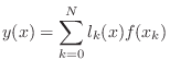
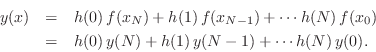
Lagrange Interpolation
Lagrange interpolation is a well known, classical technique for interpolation [193]. It is also called Waring-Lagrange interpolation, since Waring actually published it 16 years before Lagrange [309, p. 323]. More generically, the term polynomial interpolation normally refers to Lagrange interpolation. In the first-order case, it reduces to linear interpolation.
Given a set of ![]() known samples
known samples ![]() ,
,
![]() , the
problem is to find the unique order
, the
problem is to find the unique order ![]() polynomial
polynomial ![]() which
interpolates the samples.5.2The solution can be expressed as a linear combination of elementary
which
interpolates the samples.5.2The solution can be expressed as a linear combination of elementary
![]() th order polynomials:
th order polynomials:
where
![$\displaystyle l_k(x_j) = \delta_{kj} \isdef \left\{\begin{array}{ll}
1, & j=k, \\ [5pt]
0, & j\neq k. \\
\end{array}\right.
$](http://www.dsprelated.com/josimages_new/pasp/img1008.png)
![\includegraphics[width=\twidth]{eps/lagrangebases}](http://www.dsprelated.com/josimages_new/pasp/img1011.png) |
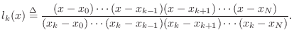
Interpolation of Uniformly Spaced Samples
In the uniformly sampled case (![]() for some sampling interval
for some sampling interval
![]() ), a Lagrange interpolator can be viewed as a Finite Impulse
Response (FIR) filter [449]. Such filters are often called
fractional delay filters
[267], since they are filters providing a non-integer time delay, in general.
Let
), a Lagrange interpolator can be viewed as a Finite Impulse
Response (FIR) filter [449]. Such filters are often called
fractional delay filters
[267], since they are filters providing a non-integer time delay, in general.
Let ![]() denote the impulse response of such a
fractional-delay filter. That is, assume the interpolation at point
denote the impulse response of such a
fractional-delay filter. That is, assume the interpolation at point
![]() is given by
is given by
where we have set ![]() for simplicity, and used the fact that
for simplicity, and used the fact that
![]() for
for
![]() in the case of ``true
interpolators'' that pass through the given samples exactly. For best
results,
in the case of ``true
interpolators'' that pass through the given samples exactly. For best
results, ![]() should be evaluated in a one-sample range centered
about
should be evaluated in a one-sample range centered
about ![]() . For delays outside the central one-sample range, the
coefficients can be shifted to translate the desired delay into
that range.
. For delays outside the central one-sample range, the
coefficients can be shifted to translate the desired delay into
that range.
Fractional Delay Filters
In fractional-delay filtering applications, the interpolator typically slides forward through time to produce a time series of interpolated values, thereby implementing a non-integer signal delay:
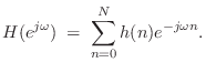
The frequency response [449] of the fractional-delay
FIR filter ![]() is
is
Lagrange Interpolation Optimality
As derived in §4.2.14, Lagrange fractional-delay filters are maximally flat in the frequency domain at dc. That is,
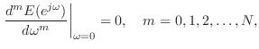
Figure 4.11 compares Lagrange and optimal Chebyshev fractional-delay
filter frequency responses. Optimality in the Chebyshev
sense means minimizing the worst-case
error over a given frequency band (in this case,
![]() ). While Chebyshev optimality is often the most desirable
choice, we do not have closed-form formulas for such solutions, so they
must be laboriously pre-calculated, tabulated, and interpolated to
produce variable-delay filtering [358].
). While Chebyshev optimality is often the most desirable
choice, we do not have closed-form formulas for such solutions, so they
must be laboriously pre-calculated, tabulated, and interpolated to
produce variable-delay filtering [358].
![\includegraphics[width=3.5in]{eps/lag}](http://www.dsprelated.com/josimages_new/pasp/img1030.png) |
Explicit Lagrange Coefficient Formulas
Given a desired fractional delay of ![]() samples, the Lagrange
fraction-delay impulse response can be written in closed form as
samples, the Lagrange
fraction-delay impulse response can be written in closed form as
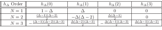
The following table gives specific examples for orders 1, 2, and 3:
Lagrange Interpolation Coefficient Symmetry
As shown in [502, §3.3.3], directly substituting into
Eq.![]() (4.7) derives the following coefficient symmetry
property for the interpolation coefficients (impulse response) of a
Lagrange fractional delay filter:
(4.7) derives the following coefficient symmetry
property for the interpolation coefficients (impulse response) of a
Lagrange fractional delay filter:
where
Matlab Code for Lagrange Interpolation
A simple matlab function for computing the coefficients of a Lagrange fractional-delay FIR filter is as follows:
function h = lagrange( N, delay )

n = 0:N;
h = ones(1,N+1);
for k = 0:N
    index = find(n ~= k);
    h(index) = h(index) *  (delay-k)./ (n(index)-k);
end
Maxima Code for Lagrange Interpolation
The maxima program is free and open-source, like Octave for matlab:5.3
  (%i1) lagrange(N, n) :=
           product(if equal(k,n) then 1
                  else (D-k)/(n-k), k, 0, N);

  (%o1) lagrange(N, n) := product(if equal(k, n) then 1

                                       D - k
                                  else -----, k, 0, N)
                                       n - k
Usage examples in maxima:
  (%i2) lagrange(1,0);
  (%o2)                             1 - D

  (%i3) lagrange(1,1);
  (%o3)                               D

  (%i4) lagrange(4,0);
                           (1 - D) (D - 4) (D - 3) (D - 2)
  (%o4)                 - -------------------------------
                                         24
  (%i5) ratsimp(lagrange(4,0));
                           4       3       2
                          D  - 10 D  + 35 D  - 50 D + 24
  (%o5)                  ------------------------------
                                      24

  (%i6) expand(lagrange(4,0));
                            4      3       2
                           D    5 D    35 D    25 D
  (%o6)                    -- - ---- + ----- - ---- + 1
                           24    12     24      12

  (%i7) expand(lagrange(4,0)), numer;
                           4                     3
  (%o7) 0.041666666666667 D  - 0.41666666666667 D
                           2
      + 1.458333333333333 D  - 2.083333333333333 D + 1.0
Faust Code for Lagrange Interpolation
The Faust programming language for signal processing [453,450] includes support for Lagrange fractional-delay filtering, up to order five, in the library file filter.lib. For example, the fourth-order case is listed below:
// fourth-order (quartic) case, delay d in [1.5,2.5]
fdelay4(n,d,x) = delay(n,id,x)   * fdm1*fdm2*fdm3*fdm4/24
               + delay(n,id+1,x) * (0-fd*fdm2*fdm3*fdm4)/6
               + delay(n,id+2,x) * fd*fdm1*fdm3*fdm4/4
               + delay(n,id+3,x) * (0-fd*fdm1*fdm2*fdm4)/6
               + delay(n,id+4,x) * fd*fdm1*fdm2*fdm3/24
with {
  o = 1.49999;
  dmo = d - o; // assumed nonnegative
  id = int(dmo);
  fd = o + frac(dmo);
  fdm1 = fd-1;
  fdm2 = fd-2;
  fdm3 = fd-3;
  fdm4 = fd-4;
};
An example calling program is shown in Fig.4.12.
// tlagrange.dsp - test Lagrange interpolation in Faust

import("filter.lib");

N = 16; % Allocated delay-line length

% Compare various orders:
D = 5.4;
process = 1-1' <: fdelay1(N,D),
                  fdelay2(N,D),
                  fdelay3(N,D),
                  fdelay4(N,D),
                  fdelay5(N,D);
// To see results:
// [in a shell]:
//   faust2octave tlagrange.dsp
// [at the Octave command prompt]:
//   plot(db(fft(faustout,1024)(1:512,:)));

// Alternate example for testing a range of 4th-order cases
// (change name to "process" and rename "process" above):
process2  = 1-1' <: fdelay4(N, 1.5),
                    fdelay4(N, 1.6),
                    fdelay4(N, 1.7),
                    fdelay4(N, 1.8),
                    fdelay4(N, 1.9),
                    fdelay4(N, 2.0),
                    fdelay4(N, 2.1),
                    fdelay4(N, 2.2),
                    fdelay4(N, 2.3),
                    fdelay4(N, 2.4),
                    fdelay4(N, 2.499),
                    fdelay4(N, 2.5);
|
Lagrange Frequency Response Examples
The following examples were generated using Faust code similar to that in Fig.4.12 and the faust2octave command distributed with Faust.
Orders 1 to 5 on a fractional delay of 0.4 samples
Figure ![]() shows the
amplitude responses of Lagrange interpolation, orders 1 through 5, for
the case of implementing an interpolated delay line of length
shows the
amplitude responses of Lagrange interpolation, orders 1 through 5, for
the case of implementing an interpolated delay line of length ![]() samples. In all cases the interpolator follows a delay line of
appropriate length so that the interpolator coefficients operate over
their central one-sample interval.
Figure
samples. In all cases the interpolator follows a delay line of
appropriate length so that the interpolator coefficients operate over
their central one-sample interval.
Figure ![]() shows the
corresponding phase delays. As discussed in §4.2.10, the
amplitude response of every odd-order case is constrained to be zero at
half the sampling rate when the delay is half-way between integers,
which this example is near. As a result, the curves for the two
even-order interpolators lie above the three odd-order interpolators at
high frequencies in
Fig.
shows the
corresponding phase delays. As discussed in §4.2.10, the
amplitude response of every odd-order case is constrained to be zero at
half the sampling rate when the delay is half-way between integers,
which this example is near. As a result, the curves for the two
even-order interpolators lie above the three odd-order interpolators at
high frequencies in
Fig.![]() . It is
also interesting to note that the 4th-order interpolator, while showing
a wider ``pass band,'' exhibits more attenuation near half the sampling
rate than the 2nd-order interpolator.
. It is
also interesting to note that the 4th-order interpolator, while showing
a wider ``pass band,'' exhibits more attenuation near half the sampling
rate than the 2nd-order interpolator.
![\includegraphics[width=0.9\twidth]{eps/tlagrange-1-to-5-ar-c}](http://www.dsprelated.com/josimages_new/pasp/img1038.png) |
![\includegraphics[width=0.9\twidth]{eps/tlagrange-1-to-5-pd-c}](http://www.dsprelated.com/josimages_new/pasp/img1039.png) |
In the phase-delay plots of
Fig.![]() , all cases
are exact at frequency zero. At half the sampling rate
they all give 5 samples of delay.
, all cases
are exact at frequency zero. At half the sampling rate
they all give 5 samples of delay.
Note that all three odd-order phase delay curves look generally better
in Fig.![]() than
both of the even-order phase delays. Recall from
Fig.
than
both of the even-order phase delays. Recall from
Fig.![]() that the
two even-order amplitude responses outperformed all three odd-order
cases. This illustrates a basic trade-off between gain accuracy and
delay accuracy. The even-order interpolators show generally less
attenuation at high frequencies (because they are not constrained to
approach a gain of zero at half the sampling rate for a half-sample
delay), but they pay for that with a relatively inferior phase-delay
performance at high frequencies.
that the
two even-order amplitude responses outperformed all three odd-order
cases. This illustrates a basic trade-off between gain accuracy and
delay accuracy. The even-order interpolators show generally less
attenuation at high frequencies (because they are not constrained to
approach a gain of zero at half the sampling rate for a half-sample
delay), but they pay for that with a relatively inferior phase-delay
performance at high frequencies.
Order 4 over a range of fractional delays
Figures 4.15 and 4.16 show amplitude response and
phase delay, respectively, for 4th-order Lagrange interpolation
evaluated over a range of requested delays from ![]() to
to ![]() samples
in increments of
samples
in increments of ![]() samples. The amplitude response is ideal (flat
at 0 dB for all frequencies) when the requested delay is
samples. The amplitude response is ideal (flat
at 0 dB for all frequencies) when the requested delay is ![]() samples
(as it is for any integer delay), while there is maximum
high-frequency attenuation when the fractional delay is half a sample.
In general, the closer the requested delay is to an integer, the
flatter the amplitude response of the Lagrange interpolator.
samples
(as it is for any integer delay), while there is maximum
high-frequency attenuation when the fractional delay is half a sample.
In general, the closer the requested delay is to an integer, the
flatter the amplitude response of the Lagrange interpolator.
![\includegraphics[width=0.9\twidth]{eps/tlagrange-4-ar}](http://www.dsprelated.com/josimages_new/pasp/img1042.png) |
![\includegraphics[width=0.9\twidth]{eps/tlagrange-4-pd}](http://www.dsprelated.com/josimages_new/pasp/img1043.png) |
Note in Fig.4.16 how the phase-delay jumps
discontinuously, as a function of delay, when approaching the desired
delay of ![]() samples from below: The top curve in
Fig.4.16 corresponds to a requested delay of 2.5
samples, while the next curve below corresponds to 2.499 samples. The
two curves roughly coincide at low frequencies (being exact at dc),
but diverge to separate integer limits at half the sampling
rate. Thus, the ``capture range'' of the integer 2 at half the
sampling rate is numerically suggested to be the half-open interval
samples from below: The top curve in
Fig.4.16 corresponds to a requested delay of 2.5
samples, while the next curve below corresponds to 2.499 samples. The
two curves roughly coincide at low frequencies (being exact at dc),
but diverge to separate integer limits at half the sampling
rate. Thus, the ``capture range'' of the integer 2 at half the
sampling rate is numerically suggested to be the half-open interval
![]() .
.
Order 5 over a range of fractional delays
Figures 4.17 and 4.18 show amplitude response and
phase delay, respectively, for 5th-order Lagrange interpolation,
evaluated over a range of requested delays between ![]() and
and ![]() samples
in steps of
samples
in steps of ![]() samples. Note that the vertical scale in
Fig.4.17 spans
samples. Note that the vertical scale in
Fig.4.17 spans ![]() dB while that in
Fig.4.15 needed less than
dB while that in
Fig.4.15 needed less than ![]() dB, again due to the
constrained zero at half the sampling rate for odd-order interpolators
at the half-sample point.
dB, again due to the
constrained zero at half the sampling rate for odd-order interpolators
at the half-sample point.
![\includegraphics[width=0.9\twidth]{eps/tlagrange-5-ar}](http://www.dsprelated.com/josimages_new/pasp/img1047.png) |
![\includegraphics[width=0.9\twidth]{eps/tlagrange-5-pd}](http://www.dsprelated.com/josimages_new/pasp/img1048.png) |
Notice in Fig.4.18 how suddenly the phase-delay curves
near 2.5 samples delay jump to an integer number of samples as a
function of frequency near half the sample rate. The curve for
![]() samples swings down to 2 samples delay, while the curve for
samples swings down to 2 samples delay, while the curve for
![]() samples goes up to 3 samples delay at half the sample rate.
Since the gain is zero at half the sample rate when the requested
delay is
samples goes up to 3 samples delay at half the sample rate.
Since the gain is zero at half the sample rate when the requested
delay is ![]() samples, the phase delay may be considered to be
exactly
samples, the phase delay may be considered to be
exactly ![]() samples at all frequencies in that special case.
samples at all frequencies in that special case.
Avoiding Discontinuities When Changing Delay
We have seen examples (e.g., Figures 4.16 and 4.18)
of the general fact that every Lagrange interpolator provides an integer
delay at frequency
![]() , except when the interpolator gain
is zero at
, except when the interpolator gain
is zero at
![]() . This is true for any interpolator
implemented as a real FIR filter, i.e., as a linear combination of signal
samples using real coefficients.5.4Therefore, to avoid a relatively large discontinuity in phase delay (at
high frequencies) when varying the delay over time, the requested
interpolation delay should stay within a half-sample range of some fixed
integer, irrespective of interpolation order. This provides that the
requested delay stays within the ``capture zone'' of a single integer at
half the sampling rate. Of course, if the delay varies by more than one
sample, there is no way to avoid the high-frequency discontinuity in the
phase delay using Lagrange interpolation.
. This is true for any interpolator
implemented as a real FIR filter, i.e., as a linear combination of signal
samples using real coefficients.5.4Therefore, to avoid a relatively large discontinuity in phase delay (at
high frequencies) when varying the delay over time, the requested
interpolation delay should stay within a half-sample range of some fixed
integer, irrespective of interpolation order. This provides that the
requested delay stays within the ``capture zone'' of a single integer at
half the sampling rate. Of course, if the delay varies by more than one
sample, there is no way to avoid the high-frequency discontinuity in the
phase delay using Lagrange interpolation.
Even-order Lagrange interpolators have an integer at the midpoint of their central one-sample range, so they spontaneously offer a one-sample variable delay free of high-frequency discontinuities.
Odd-order Lagrange interpolators, on the other hand, must be shifted by
![]() sample in either direction in order to be centered about an
integer delay. This can result in stability problems if the
interpolator is used in a feedback loop, because the interpolation gain
can exceed 1 at some frequency when venturing outside the central
one-sample range (see §4.2.11 below).
sample in either direction in order to be centered about an
integer delay. This can result in stability problems if the
interpolator is used in a feedback loop, because the interpolation gain
can exceed 1 at some frequency when venturing outside the central
one-sample range (see §4.2.11 below).
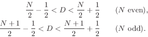
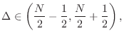
In summary, discontinuity-free interpolation ranges include
Wider delay ranges, and delay ranges not centered about an integer
delay, will include a phase discontinuity in the delay response (as a
function of delay) which is largest at frequency
![]() , as
seen in Figures 4.16 and 4.18.
, as
seen in Figures 4.16 and 4.18.
Lagrange Frequency Response Magnitude Bound
The amplitude response of fractional delay filters based on Lagrange
interpolation is observed to be bounded by 1 when the desired delay
![]() lies within half a sample of the midpoint of the coefficient
span [502, p. 92], as was the case in all preceeding examples
above. Moreover, even-order interpolators are observed to have
this boundedness property over a two-sample range centered on the
coefficient-span midpoint [502, §3.3.6]. These assertions are
easily proved for orders 1 and 2. For higher orders, a general proof
appears not to be known, and the conjecture is based on numerical
examples. Unfortunately, it has been observed that the gain of some
odd-order Lagrange interpolators do exceed 1 at some frequencies when
used outside of their central one-sample range [502, §3.3.6].
lies within half a sample of the midpoint of the coefficient
span [502, p. 92], as was the case in all preceeding examples
above. Moreover, even-order interpolators are observed to have
this boundedness property over a two-sample range centered on the
coefficient-span midpoint [502, §3.3.6]. These assertions are
easily proved for orders 1 and 2. For higher orders, a general proof
appears not to be known, and the conjecture is based on numerical
examples. Unfortunately, it has been observed that the gain of some
odd-order Lagrange interpolators do exceed 1 at some frequencies when
used outside of their central one-sample range [502, §3.3.6].
Even-Order Lagrange Interpolation Summary
We may summarize some characteristics of even-order Lagrange fractional delay filtering as follows:
- Two-sample bounded-by-1 delay-range instead of only one-sample
- No gain zero at half the sampling rate for the middle delay
- No phase-delay discontinuity when crossing the middle delay
- Optimal (central) delay range is centered about an integer
Odd-Order Lagrange Interpolation Summary
In contrast to even-order Lagrange interpolation, the odd-order case has the following properties (in fractional delay filtering applications):
- Improved phase-delay accuracy at the expense of decreased
amplitude-response accuracy (low-order examples in
Fig.
![[*]](../icons/crossref.png) )
)
- Optimal (centered) delay range lies between two integers
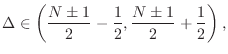
To avoid a discontinuous phase-delay jump at high frequencies when crossing the middle delay, the delay range can be shifted to
Proof of Maximum Flatness at DC
The maximumally flat fractional-delay FIR filter is obtained by equating
to zero all ![]() leading terms in the Taylor (Maclaurin) expansion of
the frequency-response error at dc:
leading terms in the Taylor (Maclaurin) expansion of
the frequency-response error at dc:
![\begin{eqnarray*}
\left\vert\left[p_i^{j-1}\right]\right\vert &=& \prod_{j>i}(p_...
...ts\\
&&(p_{N-1}-p_{N-2})(p_N-p_{N-2})\cdots\\
&&(p_N-p_{N-1}).
\end{eqnarray*}](http://www.dsprelated.com/josimages_new/pasp/img1065.png)
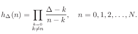
Making this substitution in the solution obtained by Cramer's rule
yields that the impulse response of the order ![]() , maximally flat,
fractional-delay FIR filter may be written in closed form as
, maximally flat,
fractional-delay FIR filter may be written in closed form as

Further details regarding the theory of Lagrange interpolation can be found (online) in [502, Ch. 3, Pt. 2, pp. 82-84].
Variable Filter Parametrizations
In practical applications of Lagrange Fractional-Delay Filtering
(LFDF), it is typically necessary to compute the FIR interpolation
coefficients
![]() as a function of the desired delay
as a function of the desired delay
![]() , which is usually time varying. Thus, LFDF is a special case
of FIR variable filtering in which the FIR coefficients must be
time-varying functions of a single delay parameter
, which is usually time varying. Thus, LFDF is a special case
of FIR variable filtering in which the FIR coefficients must be
time-varying functions of a single delay parameter ![]() .
.
Table Look-Up
A general approach to variable filtering is to tabulate the filter
coefficients as a function of the desired variables. In the case of
fractional delay filters, the impulse response
![]() is
tabulated as a function of delay
is
tabulated as a function of delay
![]() ,
,
![]() ,
,
![]() , where
, where ![]() is the
interpolation-filter order. For each
is the
interpolation-filter order. For each ![]() ,
, ![]() may be sampled
sufficiently densely so that linear interpolation will give a
sufficiently accurate ``interpolated table look-up'' of
may be sampled
sufficiently densely so that linear interpolation will give a
sufficiently accurate ``interpolated table look-up'' of
![]() for each
for each ![]() and (continuous)
and (continuous) ![]() . This method is commonly used
in closely related problem of sampling-rate conversion
[462].
. This method is commonly used
in closely related problem of sampling-rate conversion
[462].
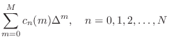
Polynomials in the Delay
A more parametric approach is to formulate each filter coefficient
![]() as a polynomial in the desired delay
as a polynomial in the desired delay ![]() :
:
Taking the z transform of this expression leads to the interesting and useful Farrow structure for variable FIR filters [134].
Farrow Structure
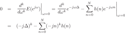
Taking the z transform of Eq.![]() (4.9) yields
(4.9) yields
![$\displaystyle \sum_{n=0}^N \left[\sum_{m=0}^M c_n(m)\Delta^m\right]z^{-n}$](http://www.dsprelated.com/josimages_new/pasp/img1079.png)
![$\displaystyle \sum_{m=0}^M \left[\sum_{n=0}^N c_n(m) z^{-n}\right]\Delta^m$](http://www.dsprelated.com/josimages_new/pasp/img1080.png)
Since
Such a parametrization of a variable filter as a polynomial in
fixed filters ![]() is called a Farrow structure
[134,502]. When the polynomial Eq.
is called a Farrow structure
[134,502]. When the polynomial Eq.![]() (4.10) is
evaluated using Horner's rule,5.5 the efficient structure of
Fig.4.19 is obtained. Derivations of Farrow-structure
coefficients for Lagrange fractional-delay filtering are introduced in
[502, §3.3.7].
(4.10) is
evaluated using Horner's rule,5.5 the efficient structure of
Fig.4.19 is obtained. Derivations of Farrow-structure
coefficients for Lagrange fractional-delay filtering are introduced in
[502, §3.3.7].
![\includegraphics[width=\twidth]{eps/farrow}](http://www.dsprelated.com/josimages_new/pasp/img1087.png) |
As we will see in the next section, Lagrange interpolation can be
implemented exactly by the Farrow structure when ![]() . For
. For ![]() ,
approximations that do not satisfy the exact interpolation property
can be computed [148].
,
approximations that do not satisfy the exact interpolation property
can be computed [148].
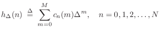
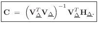
Farrow Structure Coefficients
Beginning with a restatement of Eq.![]() (4.9),
(4.9),

![$\displaystyle h_\Delta(n) \eqsp
\underbrace{%
\left[\begin{array}{ccccc} 1 & \...
...y}{c} C_n(0) \\ [2pt] C_n(1) \\ [2pt] \vdots \\ [2pt] C_n(M)\end{array}\right]
$](http://www.dsprelated.com/josimages_new/pasp/img1090.png)
![$\displaystyle \underbrace{\left[\begin{array}{cccc}h_\Delta(0)\!&\!h_\Delta(1)\...
...\vdots \\
C_0(M) & C_1(M) & \cdots & C_N(M)
\end{array}\right]}_{\mathbf{C}}
$](http://www.dsprelated.com/josimages_new/pasp/img1091.png)
where
![$\displaystyle \mathbf{H}_{\underline{\Delta}}\isdefs \left[\begin{array}{c} \un...
...elta_0}^T \\ [2pt] \vdots \\ [2pt] \underline{h}_{\Delta_L}^T\end{array}\right]$](http://www.dsprelated.com/josimages_new/pasp/img1095.png) and
and![$\displaystyle \qquad
\mathbf{V}_{\underline{\Delta}}\isdefs \left[\begin{array}...
...ta_0}^T \\ [2pt] \vdots \\ [2pt] \underline{V}_{\Delta_L}^T\end{array}\right].
$](http://www.dsprelated.com/josimages_new/pasp/img1096.png)
Differentiator Filter Bank
Since, in the time domain, a Taylor series expansion of
![]() about time
about time ![]() gives
gives
![\begin{eqnarray*}
x(n-\Delta)
&=& x(n) -\Delta\, x^\prime(n)
+ \frac{\Delta^2...
...D^2(z) + \cdots
+ \frac{(-\Delta)^k}{k!}D^k(z) + \cdots \right]
\end{eqnarray*}](http://www.dsprelated.com/josimages_new/pasp/img1101.png)
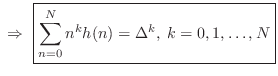
where ![]() denotes the transfer function of the ideal differentiator,
we see that the
denotes the transfer function of the ideal differentiator,
we see that the ![]() th filter in Eq.
th filter in Eq.![]() (4.10) should approach
(4.10) should approach
in the limit, as the number of terms
Farrow structures such as Fig.4.19 may be used to implement any
one-parameter filter variation in terms of several constant
filters. The same basic idea of polynomial expansion has been applied
also to time-varying filters (
![]() ).
).
Recent Developments in Lagrange Interpolation
Franck (2008) [148] provides a nice overview of the various structures being used for Lagrange interpolation, along with their computational complexities and depths (relevant to parallel processing). He moreover proposes a novel computation having linear complexity and log depth that is especially well suited for parallel processing architectures.
Relation of Lagrange to Sinc Interpolation
For an infinite number of equally spaced
samples, with spacing
![]() , the Lagrangian basis
polynomials converge to shifts of the sinc function, i.e.,
, the Lagrangian basis
polynomials converge to shifts of the sinc function, i.e.,
The equivalence of sinc interpolation to Lagrange interpolation was apparently first published by the mathematician Borel in 1899, and has been rediscovered many times since [309, p. 325].
A direct proof can be based on the equivalance between Lagrange
interpolation and windowed-sinc interpolation using a ``scaled
binomial window'' [262,502]. That is,
for a fractional sample delay of ![]() samples, multiply the
shifted-by-
samples, multiply the
shifted-by-![]() , sampled, sinc function
, sampled, sinc function
![$\displaystyle (n-D) = \frac{\sin[\pi(n-D)]}{\pi(n-D)}
$](http://www.dsprelated.com/josimages_new/pasp/img1113.png)
A more recent alternate proof appears in [557].
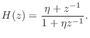
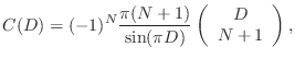
Thiran Allpass Interpolators
Given a desired delay
![]() samples, an order
samples, an order ![]() allpass filter
allpass filter
![$\displaystyle a_k=(-1)^k\left(\begin{array}{c} N \\ [2pt] k \end{array}\right)\prod_{n=0}^N\frac{\Delta-N+n}{\Delta-N+k+n},
\; k=0,1,2,\ldots,N
$](http://www.dsprelated.com/josimages_new/pasp/img1121.png)
![$\displaystyle \left(\begin{array}{c} N \\ [2pt] k \end{array}\right) = \frac{N!}{k!(N-k)!}
$](http://www.dsprelated.com/josimages_new/pasp/img1122.png)
 without further scaling
- For sufficiently large
 , stability is guaranteed
Rule of thumb:
- It can be shown that the mean group delay of any stable
th-order allpass filter is samples
[449].5.7
- Only known closed-form case for allpass interpolators of arbitrary order
- Effective for delay-line interpolation needed for tuning since pitch perception is most acute at low frequencies.
- Since Thiran allpass filters have maximally flat group-delay at dc, like Lagrange FIR interpolation filters, they can be considered the recursive extension of Lagrange interpolation.
Thiran Allpass Interpolation in Matlab
function [A,B] = thiran(D,N)
%  [A,B] = thiran(D,N)
%  returns the order N Thiran allpass interpolation filter
%  for delay D (samples).

A = zeros(1,N+1);
for k=0:N
    Ak = 1;
    for n=0:N
        Ak = Ak * (D-N+n)/(D-N+k+n);
    end
    A(k+1) = (-1)^k * nchoosek(N,k) * Ak;
end

B = A(N+1:-1:1);
Group Delays of Thiran Allpass Interpolators
Figure ![]() shows a family of
group-delay curves for Thiran allpass interpolators, for orders 1, 2,
3, 5, 10, and 20. The desired group delay was equal to the order plus
0.3 samples (which is in the ``easy zone'' for an allpass
interpolator).
shows a family of
group-delay curves for Thiran allpass interpolators, for orders 1, 2,
3, 5, 10, and 20. The desired group delay was equal to the order plus
0.3 samples (which is in the ``easy zone'' for an allpass
interpolator).
![\includegraphics[width=\twidth]{eps/thirangdC}](http://www.dsprelated.com/josimages_new/pasp/img1130.png)
Windowed Sinc Interpolation
Bandlimited interpolation of discrete-time signals is a basic tool having extensive application in digital signal processing.5.8In general, the problem is to correctly compute signal values at arbitrary continuous times from a set of discrete-time samples of the signal amplitude. In other words, we must be able to interpolate the signal between samples. Since the original signal is always assumed to be bandlimited to half the sampling rate, (otherwise aliasing distortion would occur upon sampling), Shannon's sampling theorem tells us the signal can be exactly and uniquely reconstructed for all time from its samples by bandlimited interpolation.
Considerable research has been devoted to the problem of interpolating
discrete points. A comprehensive survey of ``fractional delay filter
design'' is provided in [267]. A comparison between
classical (e.g., Lagrange) and bandlimited interpolation is given in
[407]. The book Multirate Digital Signal
Processing [97] provides a comprehensive summary and
review of classical signal processing techniques for sampling-rate
conversion. In these techniques, the signal is first interpolated by
an integer factor ![]() and then decimated by an integer factor
and then decimated by an integer factor
![]() . This provides sampling-rate conversion by any rational factor
. This provides sampling-rate conversion by any rational factor
![]() . The conversion requires a digital lowpass filter whose cutoff
frequency depends on
. The conversion requires a digital lowpass filter whose cutoff
frequency depends on
![]() . While sufficiently general, this
formulation is less convenient when it is desired to resample the
signal at arbitrary times or change the sampling-rate conversion
factor smoothly over time.
. While sufficiently general, this
formulation is less convenient when it is desired to resample the
signal at arbitrary times or change the sampling-rate conversion
factor smoothly over time.
In this section, a public-domain resampling algorithm is described which will evaluate a signal at any time specifiable by a fixed-point number. In addition, one lowpass filter is used regardless of the sampling-rate conversion factor. The algorithm effectively implements the ``analog interpretation'' of rate conversion, as discussed in [97], in which a certain lowpass-filter impulse response must be available as a continuous function. Continuity of the impulse response is simulated by linearly interpolating between samples of the impulse response stored in a table. Due to the relatively low cost of memory, the method is quite practical for hardware implementation.
In the next section, the basic theory is presented, followed by sections on implementation details and practical considerations.
Theory of Ideal Bandlimited Interpolation
We review briefly the ``analog interpretation'' of sampling rate conversion
[97] on which the present method is based. Suppose we have
samples ![]() of a continuous absolutely integrable signal
of a continuous absolutely integrable signal ![]() ,
where
,
where ![]() is time in seconds (real),
is time in seconds (real), ![]() ranges over the integers, and
ranges over the integers, and
![]() is the sampling period. We assume
is the sampling period. We assume ![]() is bandlimited to
is bandlimited to
![]() , where
, where ![]() is the sampling rate. If
is the sampling rate. If ![]() denotes the Fourier transform of
denotes the Fourier transform of ![]() , i.e.,
, i.e.,
![]() , then we assume
, then we assume
![]() for
for
![]() . Consequently, Shannon's sampling
theorem gives us that
. Consequently, Shannon's sampling
theorem gives us that ![]() can be uniquely reconstructed from the
samples
can be uniquely reconstructed from the
samples ![]() via
via
where
To resample
When the new sampling rate
![]() is less than the original rate
is less than the original rate ![]() ,
the lowpass cutoff must be placed below half the new lower sampling rate.
Thus, in the case of an ideal lowpass,
,
the lowpass cutoff must be placed below half the new lower sampling rate.
Thus, in the case of an ideal lowpass,
![]() sinc
sinc![]() , where the scale factor maintains unity gain
in the passband.
, where the scale factor maintains unity gain
in the passband.
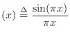
A plot of the sinc function
sinc![]() to the left and right of the origin
to the left and right of the origin ![]() is shown in Fig.4.21.
Note that peak is at amplitude
is shown in Fig.4.21.
Note that peak is at amplitude ![]() , and zero-crossings occur at all
nonzero integers. The sinc function can be seen as a hyperbolically
weighted sine function with its zero at the origin canceled out. The
name sinc function derives from its classical name as the
sine cardinal (or cardinal sine) function.
, and zero-crossings occur at all
nonzero integers. The sinc function can be seen as a hyperbolically
weighted sine function with its zero at the origin canceled out. The
name sinc function derives from its classical name as the
sine cardinal (or cardinal sine) function.
![\includegraphics[width=3in]{eps/Sinc}](http://www.dsprelated.com/josimages_new/pasp/img1149.png)
If ``![]() '' denotes the convolution operation for digital signals, then
the summation in Eq.
'' denotes the convolution operation for digital signals, then
the summation in Eq.![]() (4.13) can be written as
(4.13) can be written as
![]() .
.
Equation Eq.![]() (4.13) can be interpreted as a superpositon of
shifted and scaled sinc functions
(4.13) can be interpreted as a superpositon of
shifted and scaled sinc functions ![]() . A sinc function instance is
translated to each signal sample and scaled by that sample, and the
instances are all added together. Note that zero-crossings of
sinc
. A sinc function instance is
translated to each signal sample and scaled by that sample, and the
instances are all added together. Note that zero-crossings of
sinc![]() occur at all integers except
occur at all integers except ![]() . That means at time
. That means at time
![]() , (i.e., on a sample instant), the only contribution to the
sum is the single sample
, (i.e., on a sample instant), the only contribution to the
sum is the single sample ![]() . All other samples contribute sinc
functions which have a zero-crossing at time
. All other samples contribute sinc
functions which have a zero-crossing at time ![]() . Thus, the
interpolation goes precisely through the existing samples, as it
should.
. Thus, the
interpolation goes precisely through the existing samples, as it
should.
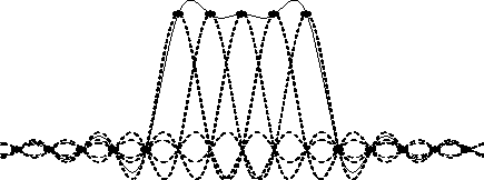
A plot indicating how sinc functions sum together to reconstruct
bandlimited signals is shown in Fig.4.22. The figure shows a
superposition of five sinc functions, each at unit amplitude, and
displaced by one-sample intervals. These sinc functions would be used
to reconstruct the bandlimited interpolation of the discrete-time
signal
![]() . Note that at each sampling
instant
. Note that at each sampling
instant ![]() , the solid line passes exactly through the tip of the
sinc function for that sample; this is just a restatement of the fact
that the interpolation passes through the existing samples. Since the
nonzero samples of the digital signal are all
, the solid line passes exactly through the tip of the
sinc function for that sample; this is just a restatement of the fact
that the interpolation passes through the existing samples. Since the
nonzero samples of the digital signal are all ![]() , we might expect the
interpolated signal to be very close to
, we might expect the
interpolated signal to be very close to ![]() over the nonzero interval;
however, this is far from being the case. The deviation from unity
between samples can be thought of as ``overshoot'' or ``ringing'' of
the lowpass filter which cuts off at half the sampling rate, or it can
be considered a ``Gibbs phenomenon'' associated with bandlimiting.
over the nonzero interval;
however, this is far from being the case. The deviation from unity
between samples can be thought of as ``overshoot'' or ``ringing'' of
the lowpass filter which cuts off at half the sampling rate, or it can
be considered a ``Gibbs phenomenon'' associated with bandlimiting.
 |
A second interpretation of Eq.![]() (4.13) is as follows: to obtain the
interpolation at time
(4.13) is as follows: to obtain the
interpolation at time ![]() , shift the signal samples under one sinc
function so that time
, shift the signal samples under one sinc
function so that time ![]() in the signal is translated under the peak of the
sinc function, then create the output as a linear combination of signal
samples where the coefficient of each signal sample is given by the value
of the sinc function at the location of each sample. That this
interpretation is equivalent to the first can be seen as a result of the
fact that convolution is commutative; in the first interpretation, all
signal samples are used to form a linear combination of shifted sinc
functions, while in the second interpretation, samples from one sinc
function are used to form a linear combination of samples of the shifted
input signal. The practical bandlimited interpolation algorithm presented
below is based on the second interpretation.
in the signal is translated under the peak of the
sinc function, then create the output as a linear combination of signal
samples where the coefficient of each signal sample is given by the value
of the sinc function at the location of each sample. That this
interpretation is equivalent to the first can be seen as a result of the
fact that convolution is commutative; in the first interpretation, all
signal samples are used to form a linear combination of shifted sinc
functions, while in the second interpretation, samples from one sinc
function are used to form a linear combination of samples of the shifted
input signal. The practical bandlimited interpolation algorithm presented
below is based on the second interpretation.
From Theory to Practice
The summation in Eq.![]() (4.13) cannot be implemented in practice because
the ``ideal lowpass filter'' impulse response
(4.13) cannot be implemented in practice because
the ``ideal lowpass filter'' impulse response ![]() actually extends
from minus infinity to infinity. It is necessary in practice to window the ideal impulse response so as to make it finite. This is the basis
of the window method for digital filter design
[115,362]. While many other filter design techniques
exist, the window method is simple and robust, especially for very
long impulse responses. In the case of the algorithm presented below,
the filter impulse response is very long because it is heavily
oversampled. Another approach is to design optimal decimated
``sub-phases'' of the filter impulse response, which are then
interpolated to provide the ``continuous'' impulse response needed for
the algorithm [358].
actually extends
from minus infinity to infinity. It is necessary in practice to window the ideal impulse response so as to make it finite. This is the basis
of the window method for digital filter design
[115,362]. While many other filter design techniques
exist, the window method is simple and robust, especially for very
long impulse responses. In the case of the algorithm presented below,
the filter impulse response is very long because it is heavily
oversampled. Another approach is to design optimal decimated
``sub-phases'' of the filter impulse response, which are then
interpolated to provide the ``continuous'' impulse response needed for
the algorithm [358].
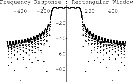
Figure 4.23 shows the frequency response of the ideal
lowpass filter. This is just the Fourier transform of ![]() .
.

If we truncate ![]() at the fifth zero-crossing to the left and the
right of the origin, we obtain the frequency response shown in
Fig.4.24. Note that the stopband exhibits only slightly
more than 20 dB rejection.
at the fifth zero-crossing to the left and the
right of the origin, we obtain the frequency response shown in
Fig.4.24. Note that the stopband exhibits only slightly
more than 20 dB rejection.
 |
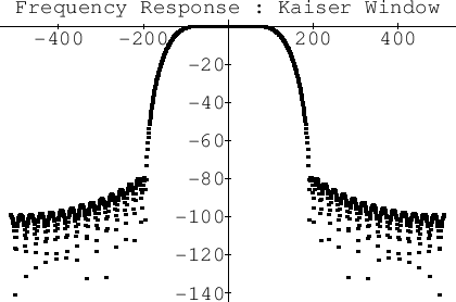
If we instead use the Kaiser window [221,438] to
taper ![]() to zero by the fifth zero-crossing to the left and the
right of the origin, we obtain the frequency response shown in
Fig.4.25. Note that now the stopband starts out close to
to zero by the fifth zero-crossing to the left and the
right of the origin, we obtain the frequency response shown in
Fig.4.25. Note that now the stopband starts out close to
![]() dB. The Kaiser window has a single parameter which can be used
to modify the stop-band attenuation, trading it against the transition
width from pass-band to stop-band.
dB. The Kaiser window has a single parameter which can be used
to modify the stop-band attenuation, trading it against the transition
width from pass-band to stop-band.
 |
Implementation
The implementation below provides signal evaluation at an arbitrary time, where time is specified as an unsigned binary fixed-point number in units of the input sampling period (assumed constant).
![\includegraphics[scale=0.8]{eps/TimeRegisterFormat}](http://www.dsprelated.com/josimages_new/pasp/img1160.png)
![\includegraphics[scale=0.8]{eps/Waveforms}](http://www.dsprelated.com/josimages_new/pasp/img1161.png)
Figure 4.26 shows the time register ![]() , and
Figure 4.27 shows an example configuration of the input
signal and lowpass filter at a given time. The time register is
divided into three fields: The leftmost field gives the number
, and
Figure 4.27 shows an example configuration of the input
signal and lowpass filter at a given time. The time register is
divided into three fields: The leftmost field gives the number ![]() of
samples into the input signal buffer, the middle field is an initial
index
of
samples into the input signal buffer, the middle field is an initial
index ![]() into the filter coefficient table
into the filter coefficient table ![]() , and the rightmost
field is interpreted as a number
, and the rightmost
field is interpreted as a number ![]() between 0 and
between 0 and ![]() for doing
linear interpolation between samples
for doing
linear interpolation between samples ![]() and
and ![]() (initially) of the
filter table. The concatenation of
(initially) of the
filter table. The concatenation of ![]() and
and ![]() are called
are called
![]() which is interpreted as the position of the current time
between samples
which is interpreted as the position of the current time
between samples ![]() and
and ![]() of the input signal.
of the input signal.
Let the three fields have ![]() ,
, ![]() , and
, and ![]() bits,
respectively. Then the input signal buffer contains
bits,
respectively. Then the input signal buffer contains ![]() samples, and the filter table contains
samples, and the filter table contains ![]() ``samples per
zero-crossing.'' (The term ``zero-crossing'' is precise only for the case
of the ideal lowpass; to cover practical cases we generalize
``zero-crossing'' to mean a multiple of time
``samples per
zero-crossing.'' (The term ``zero-crossing'' is precise only for the case
of the ideal lowpass; to cover practical cases we generalize
``zero-crossing'' to mean a multiple of time
![]() , where
, where ![]() is the lowpass cutoff frequency.) For example, to use the ideal lowpass
filter, the table would contain
is the lowpass cutoff frequency.) For example, to use the ideal lowpass
filter, the table would contain
![]() sinc
sinc![]() .
.
Our implementation stores only the ``right wing'' of a symmetric
finite-impulse-response (FIR) filter (designed by the window method
based on a Kaiser window [362]). Specifically, if
![]() ,
,
![]() , denotes a length
, denotes a length ![]() symmetric
finite impulse response, then the
right wing
of
symmetric
finite impulse response, then the
right wing
of ![]() is defined
as the set of samples
is defined
as the set of samples ![]() for
for
![]() . By symmetry, the
left wing can be reconstructed as
. By symmetry, the
left wing can be reconstructed as
![]() ,
,
![]() .
.
Our implementation also stores a table of differences
![]() between successive FIR sample values in order to
speed up the linear interpolation. The length of each table is
between successive FIR sample values in order to
speed up the linear interpolation. The length of each table is
![]() , including the endpoint definition
, including the endpoint definition
![]() .
.
Consider a sampling-rate conversion by the factor
![]() .
For each output sample, the basic interpolation Eq.
.
For each output sample, the basic interpolation Eq.![]() (4.13) is
performed. The filter table is traversed twice--first to apply the
left wing of the FIR filter, and second to apply the right wing.
After each output sample is computed, the time register is incremented
by
(4.13) is
performed. The filter table is traversed twice--first to apply the
left wing of the FIR filter, and second to apply the right wing.
After each output sample is computed, the time register is incremented
by
![]() (i.e., time is incremented by
(i.e., time is incremented by ![]() in
fixed-point format). Suppose the time register
in
fixed-point format). Suppose the time register ![]() has just been
updated, and an interpolated output
has just been
updated, and an interpolated output ![]() is desired. For
is desired. For
![]() , output is computed via
, output is computed via
![\begin{eqnarray*}
v & \gets & \sum_{i=0}^{\mbox{$h$\ end}} x(n-i) \left[h(l+iL) ...
...$\ end}}
x(n+1+i) \left[h(l+iL) + \epsilon \hbar(l+iL)\right],
\end{eqnarray*}](http://www.dsprelated.com/josimages_new/pasp/img1186.png)
where ![]() is the current input sample, and
is the current input sample, and
![]() is the
interpolation factor. When
is the
interpolation factor. When ![]() , the initial
, the initial ![]() is replaced by
is replaced by
![]() ,
, ![]() becomes
becomes
![]() , and the
step-size through the filter table is reduced to
, and the
step-size through the filter table is reduced to ![]() instead of
instead of
![]() ; this lowers the filter cutoff to avoid aliasing. Note that
; this lowers the filter cutoff to avoid aliasing. Note that ![]() is fixed throughout the computation of an output sample when
is fixed throughout the computation of an output sample when
![]() but changes when
but changes when ![]() .
.
When ![]() , more input samples are required to reach the end of the
filter table, thus preserving the filtering quality. The number of
multiply-adds per second is approximately
, more input samples are required to reach the end of the
filter table, thus preserving the filtering quality. The number of
multiply-adds per second is approximately
![]() .
Thus the higher sampling rate determines the work rate. Note that for
.
Thus the higher sampling rate determines the work rate. Note that for
![]() there must be
there must be
![]() extra input samples
available before the initial conversion time and after the final conversion
time in the input buffer. As
extra input samples
available before the initial conversion time and after the final conversion
time in the input buffer. As ![]() , the required extra input
data becomes infinite, and some limit must be chosen, thus setting a
minimum supported
, the required extra input
data becomes infinite, and some limit must be chosen, thus setting a
minimum supported
![]() . For
. For ![]() , only
, only ![]() extra input samples are required on
the left and right of the data to be resampled, and the upper bound for
extra input samples are required on
the left and right of the data to be resampled, and the upper bound for
![]() is determined only by the fixed-point number format, viz.,
is determined only by the fixed-point number format, viz.,
![]() .
.
As shown below, if ![]() denotes the word-length of the stored
impulse-response samples, then one may choose
denotes the word-length of the stored
impulse-response samples, then one may choose ![]() , and
, and
![]() to obtain
to obtain ![]() effective bits of precision in the
interpolated impulse response.
effective bits of precision in the
interpolated impulse response.
Note that rational conversion factors of the form ![]() , where
, where
![]() and
and ![]() is an arbitrary positive integer, do not use the linear
interpolation feature (because
is an arbitrary positive integer, do not use the linear
interpolation feature (because
![]() ). In this case our method reduces
to the normal type of bandlimited interpolator [97]. With the
availability of interpolated lookup, however, the range of conversion
factors is boosted to the order of
). In this case our method reduces
to the normal type of bandlimited interpolator [97]. With the
availability of interpolated lookup, however, the range of conversion
factors is boosted to the order of
![]() . E.g., for
. E.g., for
![]() ,
,
![]() , this is about
, this is about ![]() decimal digits of
accuracy in the conversion factor
decimal digits of
accuracy in the conversion factor ![]() . Without interpolation, the
number of significant figures in
. Without interpolation, the
number of significant figures in ![]() is only about
is only about ![]() .
.
The number ![]() of zero-crossings stored in the table is an independent
design parameter. For a given quality specification in terms of aliasing
rejection, a trade-off exists between
of zero-crossings stored in the table is an independent
design parameter. For a given quality specification in terms of aliasing
rejection, a trade-off exists between ![]() and sacrificed bandwidth.
The lost bandwidth is due to the so-called ``transition band'' of the
lowpass filter [362]. In general, for a given stop-band
specification (such as ``80 dB attenuation''), lowpass filters need
approximately twice as many multiply-adds per sample for each halving of
the transition band width.
and sacrificed bandwidth.
The lost bandwidth is due to the so-called ``transition band'' of the
lowpass filter [362]. In general, for a given stop-band
specification (such as ``80 dB attenuation''), lowpass filters need
approximately twice as many multiply-adds per sample for each halving of
the transition band width.
As a practical design example, we use ![]() in a system designed for
high audio quality at
in a system designed for
high audio quality at ![]() % oversampling. Thus, the effective FIR
filter is
% oversampling. Thus, the effective FIR
filter is ![]() zero crossings long. The sampling rate in this case would
be
zero crossings long. The sampling rate in this case would
be ![]() kHz.5.9In the most straightforward filter design, the lowpass filter pass-band
would stop and the transition-band would begin at
kHz.5.9In the most straightforward filter design, the lowpass filter pass-band
would stop and the transition-band would begin at ![]() kHz, and the
stop-band would begin (and end) at
kHz, and the
stop-band would begin (and end) at ![]() kHz. As a further refinement,
which reduces the filter design requirements, the transition band is really
designed to extend from
kHz. As a further refinement,
which reduces the filter design requirements, the transition band is really
designed to extend from ![]() kHz to
kHz to ![]() kHz, so that the half of it
between
kHz, so that the half of it
between ![]() and
and ![]() kHz aliases on top of the half between
kHz aliases on top of the half between ![]() and
and ![]() kHz, thereby approximately halving the filter length required. Since the
entire transition band lies above the range of human hearing, aliasing
within it is not audible.
kHz, thereby approximately halving the filter length required. Since the
entire transition band lies above the range of human hearing, aliasing
within it is not audible.
Using ![]() samples per zero-crossing in the filter table for the above
example (which is what we use at CCRMA, and which is somewhat over
designed) implies desiging a length
samples per zero-crossing in the filter table for the above
example (which is what we use at CCRMA, and which is somewhat over
designed) implies desiging a length
![]() FIR filter
having a cut-off frequency near
FIR filter
having a cut-off frequency near ![]() . It turns out that optimal
Chebyshev design procedures such as the Remez multiple exchange algorithm
used in the Parks-McLellan software
[362] can only handle filter lengths up to a couple hundred
or so. It is therefore necessary to use an FIR filter design method which
works well at such very high orders, and the window method employed here is
one such method.
. It turns out that optimal
Chebyshev design procedures such as the Remez multiple exchange algorithm
used in the Parks-McLellan software
[362] can only handle filter lengths up to a couple hundred
or so. It is therefore necessary to use an FIR filter design method which
works well at such very high orders, and the window method employed here is
one such method.
It is worth noting that a given percentage increase in the original
sampling rate (``oversampling'') gives a larger percentage savings in
filter computation time, for a given quality specification, because the
added bandwidth is a larger percentage of the filter transition bandwidth
than it is of the original sampling rate. For example, given a cut-off
frequency of ![]() kHz, (ideal for audio work), the transition band
available with a sampling rate of
kHz, (ideal for audio work), the transition band
available with a sampling rate of ![]() kHz is about
kHz is about ![]() kHz, while a
kHz, while a
![]() kHz sampling rate provides a
kHz sampling rate provides a ![]() kHz transition band. Thus, a
kHz transition band. Thus, a
![]() % increase in sampling rate halves the work per sample in
the digital lowpass filter.
% increase in sampling rate halves the work per sample in
the digital lowpass filter.
Choice of Table Size and Word Lengths
It is desirable that the stored filter impulse response be sampled
sufficiently densely so that interpolating linearly between samples
does not introduce error greater than the quantization error. It is
shown in [462] that this condition is satisfied
when the filter impulse-response table contains at least
![]() entries per ``zero-crossing'', where
entries per ``zero-crossing'', where ![]() is the
number of bits allocated to each table entry. (A later, sharper,
error bound gives that
is the
number of bits allocated to each table entry. (A later, sharper,
error bound gives that
![]() is sufficient.) It is
additionally shown in [462] that the number of bits in the interpolation
between impulse-response samples should be near
is sufficient.) It is
additionally shown in [462] that the number of bits in the interpolation
between impulse-response samples should be near ![]() or more. With these
choices, the linear interpolation error and the error due to quantized
interpolation factors are each about equal to the coefficient
quantization error. A signal resampler designed according to these
rules will typically be limited primarily by the lowpass filter
design, rather than by quantization effects.
or more. With these
choices, the linear interpolation error and the error due to quantized
interpolation factors are each about equal to the coefficient
quantization error. A signal resampler designed according to these
rules will typically be limited primarily by the lowpass filter
design, rather than by quantization effects.
Summary of Windowed Sinc Interpolation
The digital resampling method described in this section is convenient for bandlimited interpolation of discrete-time signals at arbitrary times and/or for arbitrary changes in sampling rate. The method is well suited for software or hardware implementation, and widely used free software is available.
Delay-Line Interpolation Summary
The most commonly used closed-form methods for delay-line interpolation may be summarized by the following table:
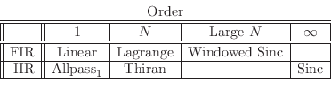
In the second column -- ![]() th-order interpolation -- we list
Lagrange for the FIR case (top) and Thiran for the IIR case (bottom),
and these are introduced in §4.2 and §4.3,
respectively. Lagrange and Thiran interpolators, properly
implemented, enjoy the following advantages:
th-order interpolation -- we list
Lagrange for the FIR case (top) and Thiran for the IIR case (bottom),
and these are introduced in §4.2 and §4.3,
respectively. Lagrange and Thiran interpolators, properly
implemented, enjoy the following advantages:
- Gain bounded by 1 at all frequencies
- Coefficients known in closed form as a function of desired delay
- Maximally flat at low frequencies:
- -
- Lagrange: maximally flat frequency response at dc
- -
- Thiran: maximally flat group delay at dc
In the high-order FIR case, one should also consider ``windowed sinc'' interpolation (introduced in §4.4) as an alternative to Lagrange interpolation. In fact, as discussed in §4.2.16, Lagrange interpolation is a special case of windowed-sinc interpolation in which a scaled binomial window is used. By choosing different windows, optimalities other than ``maximally flat at dc'' can be achieved.
In the most general ![]() th-order case, the interpolation-filter impulse
response may be designed to achieve any optimality objective, such as
Chebyshev optimality (Fig.4.11). That is, design a digital filter
(FIR or IIR) that approximates
th-order case, the interpolation-filter impulse
response may be designed to achieve any optimality objective, such as
Chebyshev optimality (Fig.4.11). That is, design a digital filter
(FIR or IIR) that approximates
FIR interpolators have the advantage that they can be used in ``random access'' mode. IIR interpolators, on the other hand, require a sequential stream of input samples and produce a sequential stream of interpolated signal samples (typically implementing a fractional delay). In IIR fractional-delay filters, the fractional delay must change slowly relative to the IIR duration.
Finally, we note in the last column of the above table that if ``order
is no object'' (
![]() ), then the ideal bandlimited-interpolator
impulse-response is simply a sampled
sinc function, as discussed in
§4.4.
), then the ideal bandlimited-interpolator
impulse-response is simply a sampled
sinc function, as discussed in
§4.4.
Next Section:
Time-Varying Delay Effects
Previous Section:
Artificial Reverberation


