I have tried both autocorrelation and a simple FFT power spectrum, but I cannot see how I can extract the tone of this audio signal:

www.tunelab-world.com/irregular-engine.wav

I can hear a tone with my ears, and by matching with a signal generator I know it is around 190 Hz. The sound is from a chain saw engine operating in a mode where the RPM is being controlled by controlled misfires from suppressing the spark. This creates a very unstable signal with wide "peaks" in the power spectrum. I have also looked at the time series data and there is no obvious pattern there either. However my ears tell me the average RPM is quite stable. I can specify that in the actual application, the pitch will always be between 120 Hz and 240 Hz. Using that knowledge, is there any hope of my extracting a pitch with an algorithm?

Bob Scott
Hopkins, MN

I just built a musical instrument tuner that's based on phase vocoder principles and it seems to work pretty well on irregular waveforms for estimating frequency. The process involves:

* A short-time Fourier Transform built with an overlap/save process and a Hann window. I use a hop-size of 8.

* Convert the I/Q bins to polar

* Do a peak search on magnitude and find a peak that persists for more than one transform.

* Once the peak is found, use the phase information to extract frequency. This means differentiating the phase between successive transforms. Since the STFT acts like a filter bank, the phase of any bin will precess at a rate determined by any tone that falls within that bin. There are some "fun" phase unwrapping tricks needed, and you'll have to offset the resulting frequency by the center frequency of the bin.

* Note that if the peak response in the STFT is not the fundamental then the frequency estimate may be off by an octave. This isn't a huge problem for my instrument tuner because I care more about the note within the octave. For more accurate fundamental estimation you might need to search for the lowest frequency peak, not merely the highest magnitude peak overall. 

It's a bit involved, but it seems to estimate the frequency correctly after only two or three frames of the STFT. Filtering the estimate seems to help a bit too. End result is estimates that are good to better than 0.1Hz with a 1k FFT running at 48kHz.

When you say "irregular waveforms" do you mean severely aperiodic?  Have you listened to the audio clip I posted, and does it sound like what you method has worked on?

Yes, I grabbed the clip you posted and listened to it. I also looked at it in time & frequency with Audacity. It seems to have a fairly strong peak around 377Hz which my algorithm would likely be able to lock onto and estimate.

A possibility of a next thing to do, since you know the frequency range of interest, is to filter out everything but that range.  i.e., isolate the 120-240Hz spectrum with a good time-domain filter, maybe with some interpolation from the bandwidth reduction to increase the number of samples.   That may help with FT analysis, or it may increase samples enough that a time-domain algorithm like Kay's method may be useful.

This sort of analysis is inherently difficult.  There are apparently reasonably reliable music analyzers that can pick out a melody from a YouTube video and send you a copyright notice...this happens to me.  ;)    So there may be better algorithms, but if it were me I'd try the above and see if it gets better or gives you more ideas.

What is your audio sample rate?  How many samples in the source material? What kind of windowing are you using?  Would you be willing to share the results of your autocorrelation and power spectrum attempts (ie images of the plots)?

Windowing and making sure you have enough data would be key in making this work with one of those schemes, and I’d guess they’d be your best bet

The sample rate for analysis is 44,100 sps.  It is DC-centered and there is a slight amount of trapezoidal windowing - a ramp up at the beginning and a ramp down at the end, comprising 1/16 of the sample period at each end.  The autocorrelation scheme works very well when the engine is being controlled by a throttle and not by random misfires.  Here is an example of the autocorrelation graph when the engine is running smoothly at about 133 revs per second:

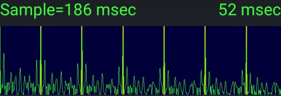
The autocorrelation graph is in green.  The yellow lines are placed by my analysis software as it locates the peaks in that graph.  The sample period is 186 msec. and the graph is currently scaled horizontally to show everything up to 52 msec.  As expected, there are 6 peaks visible in the first 52 msec., since 133 pulses per second means 7.5 msec. per peak.  Now look the autocorrelation graph for 190 revs per second where irregular ignition is causing phase noise and random amplitude modulation:

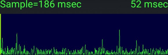
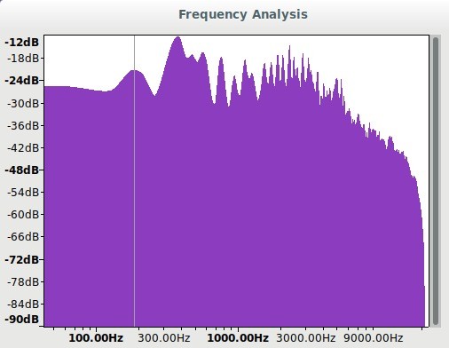
It looks like total garbage.  At 190 pulses per second we would expect to see about 9 or 10 peaks in this range.  This was made from the same audio clip I posted in by original posting.  And here is a simple FFT power spectrum of the same clip:

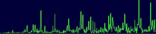
The sample period is the same 186 msec. The right side of the graph is approximately 1750 Hz, so it includes the fundamental of 190 Hz and about the first 9 harmonics.  I sort of see it, but there is so much noise I don't see how I could extract the fundamental reliably.  By contrast, here is the power spectrum of the smoothly running engine without ignition skipping, running at 133 revs per sec.:

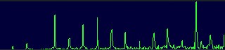
Finding the fundamental in this graph is a piece of cake.  I am tempted to say that it is impossible to extract the pitch of the irregular engine, but my ears hear it so very easily that perhaps there is a way.

For human sound analysis, there are a lot of algorithms based on autocorrelation or frequency spectrum for "pitch estimation". spectrum.jpeg Looking at spectrum, I see peaks at 185 and 370 Hz. Hence 185 Hz seems to be your value. 

These are some very interesting ideas.  I wonder if perhaps I have an error in my implementation of autocorrelation because it is not at all obvious from the graph of autocorrelation I posted how one might extract pitch from it.  The simple FFT actually looks more promising, perhaps if preceded by some time-domain filtering.

My application is a mobile app for Android and iOS.  I really don't want to import some third-party library if I can write the code from first principles.  I already have a very efficient FFT, and the autocorrelation code uses two FFT calculations separated by some real and imaginary part shuffling that I found in a source of DSP algorithms.  It has worked very well, giving me exactly what I would expect in the graph for all sorts of periodic signals.  It only in this one with so much phase noise and amplitude modulation that the results look meaningless.  But if these other software packages can do, I will look again and see if I can do it in my code.

Thanks to everybody for all the advice.  I used to be in the DSP usenet newsgroup many years ago before it migrated to web site format.  I even recognize some of the names here from that old group.

-Bob Scott

Hopkins, MN

I used autocorrelation (in Pyton, used librosa library) with the restriction that 120-240 Hz is the range for pitch find range. 

import numpy, scipy, matplotlib.pyplot as plt, IPython.display as ipd
import librosa, librosa.display
x, sr = librosa.load('irregular-engine.wav', sr=44100, mono=False)
r = librosa.autocorrelate(x[0,:], max_size=5000)
f_hi = 240
f_lo = 120
t_lo = sr/f_hi
t_hi = sr/f_lo
r[:int(t_lo)] = 0
r[int(t_hi):] = 0
t_max = r.argmax()

print(float(sr)/t_max)

That gave 191 Hz (actually a little different from power spectrum analysis I sent previously, that was 185 Hz)

Hello,

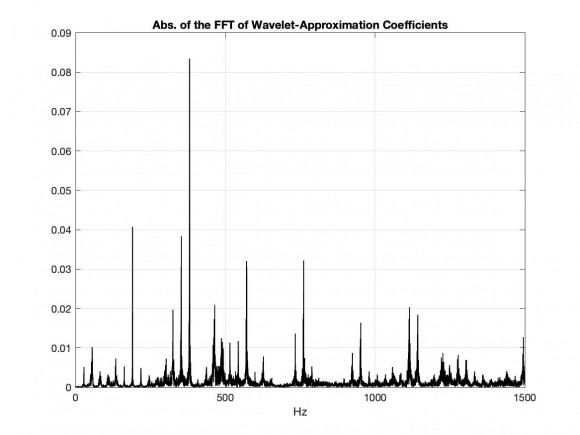
I tried to analyze your wav file with a wavelet transform. With two stages, the approximation coefficients are freed from interference, giving the pitch frequency in the FFT of the approximation coefficients.

My MATLAB script is:

% Script pitch_2.m, in which the Pitch-Freq. is determined using

% the Wavelet-Transformation

clear;

% ------- Reading the wav file 

[y,fs] = audioread('irregular-engine.wav');

ny = length(y(:,1));

Ts = 1/fs;

t = 0:Ts:(ny-1)*Ts;

figure(1);   clf;

plot(t,y(:,1),'-k','LineWidth',1);

La = axis;   axis([0.5,1,La(3:4)]);

title('Signal');

xlabel('Time in s');   grid on;

% ------ Wavelet Transformation first stage

[ca,cd] = dwt(y(:,1), 'db4');

na = length(ca);

figure(2);   clf;

subplot(211), plot(0:na-1, ca,'-k','LineWidth',1);

title('Approximation-Coefficients');

subplot(212), plot(0:na-1, cd,'-k','LineWidth',1);

title('Details-Coefficients');

% ------ Wavelet-Transformation second stage

[ca1,cd1] = dwt(ca, 'db4');

na1 = length(ca1);

CA1 = fft(ca1)/na1;     % FFT of the Approximation-Coefficients

CD1 = fft(cd1)/na1;     % FFT of the Details-Coefficients

figure(3);    clf;

plot((0:na1-1)*(fs/4)/na1, abs(CA1),'-k','LineWidth',1);

La = axis;    axis([0,1500,La(3:4)]);

title('Abs. of the FFT of Wavelet-Approximation Coefficients');

xlabel('Hz');   grid;

n_ca1_max = find(abs(CA1) == max(abs(CA1))),

fpitch = (n_ca1_max(1)-1)*(fs/4)/na1,    % The Freq. of the FFT pick

%################## 

The result is 380.6940 Hz

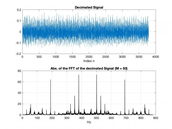
% ------ The solution with filtering and decimation

nord = 128;

M = 50;                 % Decimation factor

h = fir1(nord, 1/M);  % Decimation FIR Filter

y1 = filter(h,1,y);

y1d = y1(1:M:end);     

ny1d = length(y1d);

Y1d = fft(y1d);

figure(4);    clf;

subplot(211), plot(0:ny1d-1, y1d);

title('Decimated Signal')

xlabel('Index n');  grid on

subplot(212), plot((0:ny1d-1)*(fs/50)/ny1d, abs(Y1d),...

'-k','LineWidth',1);

title(['Abs. of the FFT of the decimated Signal (M = 50)']);

xlabel('Hz');   grid;

FYI, when sharing code, you can take advantage of the highlighter by selecting your code and then click on the 'formatting' button and select 'Code':

% Script pitch_2.m, in which the Pitch-Freq. is determined using

% the Wavelet-Transformation

clear;

% ------- Reading the wav file 

[y,fs] = audioread('irregular-engine.wav');

ny = length(y(:,1));

Ts = 1/fs;

t = 0:Ts:(ny-1)*Ts;

figure(1);   clf;

plot(t,y(:,1),'-k','LineWidth',1);

La = axis;   axis([0.5,1,La(3:4)]);

title('Signal');

xlabel('Time in s');   grid on;

% ------ Wavelet Transformation first stage

[ca,cd] = dwt(y(:,1), 'db4');

na = length(ca);

figure(2);   clf;

subplot(211), plot(0:na-1, ca,'-k','LineWidth',1);

title('Approximation-Coefficients');

subplot(212), plot(0:na-1, cd,'-k','LineWidth',1);

title('Details-Coefficients');

% ------ Wavelet-Transformation second stage

[ca1,cd1] = dwt(ca, 'db4');

na1 = length(ca1);

CA1 = fft(ca1)/na1;     % FFT of the Approximation-Coefficients

CD1 = fft(cd1)/na1;     % FFT of the Details-Coefficients

figure(3);    clf;

plot((0:na1-1)*(fs/4)/na1, abs(CA1),'-k','LineWidth',1);

La = axis;    axis([0,1500,La(3:4)]);

title('Abs. of the FFT of Wavelet-Approximation Coefficients');

xlabel('Hz');   grid;

n_ca1_max = find(abs(CA1) == max(abs(CA1))),

fpitch = (n_ca1_max(1)-1)*(fs/4)/na1,    % The Freq. of the FFT pick

%##################

This is also a very nice approach, eliminating noise. I also found (also in this thread a sent) 380 Hz but there is a previous peak at 185-190 Hz. That is the desired frequency I think, but your approach is better for removing noise. Two first dominant frequencies could be found in your code (n_ca1_max = find(abs(CA1) == max(abs(CA1))) )

The second frequency is just the reflection of the first frequency in the second Nyquist interval !

Your plot also reflects peaks at harmonics of ~185 Hz.  380 Hz is one of them. (Fs=44100 Hz, good enough for resolution - not a reflection case here)

The plot is only a section at the beginning of the FFT !

If you look at the tunelabguy's plots above, he confirms indeed fundamental frequency around 190 Hz and its 9 harmonics. YOur plot is also in this way, confirming it also.

Hello,

If Matlab is available to you, you may want to explore the Mustafa and Bruce (2006) formant tracker.

The estimated pitch is 150 Hz, which agrees with your qualitative pitch range of 120 Hz to 240 Hz.  See the image below.  I have added a data-tip in the plot to label the pitch.

Based on spectral analysis, I observed a peak at approximately 380 Hz.  A value similar to what others here have produced.

The link provides a secondary link to the paper describing its functionaility.

I wonder if cepstrum analysis might be suitable for this task, ala:

http://people.ee.ethz.ch/~spr/f0_detection/