Loop Filter Identification

Free Books Physical Audio Signal Processing

In §6.7 we discussed damping filters for vibrating string models, and in §6.9 we discussed dispersion filters. For vibrating strings which are well described by a linear, time-invariant (LTI) partial differential equation, damping and dispersion filtering are the only deviations possible from the ideal string string discussed in §6.1.

The ideal damping filter is ``zero phase'' (or linear phase) [449],^7.10while the ideal dispersion filter is ``allpass'' (as described in §6.9.1). Since every desired frequency response can be decomposed into a zero-phase frequency-response in series with an allpass frequency-response, we may design a single loop filter whose amplitude response gives the desired damping as a function of frequency, and whose phase response gives the desired dispersion vs. frequency. The next subsection summarizes some methods based on this approach. The following two subsections discuss methods for the design of damping and dispersion filters separately.

General Loop-Filter Design

For general loop-filter design in vibrating string models (as well as in woodwind and brass instrument bore models), we wish to minimize [428, pp. 182-184]:

Errors in partial overtone decay times
Errors in partial overtone tuning

The partial decay times are controlled by the filter's amplitude response, while the partial tunings are determined by the filter's phase response. There also may be other filters in the loop (such as a delay-line interpolation filter) which need to be considered when designing the main loop filter.

There are numerous methods for designing the string loop filter ${\hat G}(z)$ based on measurements of real string behavior. In [428], a variety of methods for system identification [288] were explored for this purpose, including ``periodic linear prediction'' in which a linear combination of a small group of samples is used to predict a sample one period away from the midpoint of the group. An approach based on a genetic algorithm is described in [378]; in that work, the error measure used with the genetic algorithm is based on properties of human perception of short-time spectra, as is now standard practice in digital audio coding [62]. Overviews of other approaches appear in [29] and [508].

Below is an outline of a simple and effective method used (ca. 1995) to design loop filters for some of the Sondius sound examples:

Estimate the fundamental frequency (see §6.11.4 below)
Set a Hamming FFT-window length to approximately four periods
Compute the short-time Fourier transform (STFT)
Perform a sinusoidal modeling analysis [466] to

-

detect peaks in each spectral frame, and

-

connect peaks through time to form amplitude envelopes
Fit an exponential to each amplitude envelope
Prepare the desired frequency-response, sampled at the harmonic frequencies of the delay-line loop without the loop filter. At each harmonic frequency,

-

the nearest-partial decay-rate gives the desired loop-filter gains,

-

the nearest-partial peak-frequency give the desired loop-filter phase delay.
Use a phase-sensitive filter-design method such as invfreqz in matlab to design the desired loop filter from its frequency-response samples (further details below).

Physically, amplitude envelopes are expected to decay exponentially, although coupling phenomena may obscure the overall exponential trend. On a dB scale, exponential decay is a straight line. Therefore, a simple method of estimating the exponential decay time-constant for each overtone frequency is to fit a straight line to its amplitude envelope and use the slope of the fitted line to compute the decay time-constant. For example, the matlab function polyfit can be used for this purpose (where the requested polynomial order is set to 1). Since ``beating'' is typical in the amplitude envelopes, a refinement is to replace the raw amplitude envelope by a piecewise linear envelope that connects the upper local maxima in the raw amplitude envelope. The estimated decay-rate for each overtone determines a sample of the loop-filter amplitude response at the overtone frequency. Similarly, the overtone frequency determines a sample of the loop-filter phase response.

Taken together, the measured overtone decay rates and tunings determine samples of the complex frequency response of the desired loop filter. The matlab function invfreqz^7.11 can be used to convert these complex samples into recursive filter coefficients (see §8.6.4 for a related example). A weighting function inversely proportional to frequency is recommended. Additionally, Steiglitz-McBride iterations can improve the results [287], [428, pp. 101-103]. Matlab's version of invfreqz has an iteration-count argument for specifying the number of Steiglitz-McBride iterations. The maximum filter-gain versus frequency should be computed, and the filter should be renormalized, if necessary, to ensure that its gain does not exceed 1 at any frequency; one good setting is that which matches the overall decay rate of the original recording.

Damping Filter Design

When dispersion can be neglected (as it typically can in many cases, such as for guitar strings), we may use linear-phase filter design methods, such as provided by the functions remez, firls, and fir2 in matlab. Since strings are usually very lightly damped, such linear-phase filter designs give high quality at very low orders. Another approach is to fit a low-order IIR filter, such as by applying invfreqz to a minimum-phase version of the desired amplitude response, and then subtract the phase-response of the resulting filter from the desired phase-response used in a subsequent allpass design. (Alternatively, the phase response of the loop filter can simply be neglected, as long as tuning is unaffected. If tuning is affected, the tuning allpass can be adjusted to compensate.)

Dispersion Filter Design

A pure dispersion filter is an ideal allpass filter. That is, it has a gain of 1 at all frequencies and only delays a signal in a frequency-dependent manner. The need for such filtering in piano string models is discussed in §9.4.1.

There is a good amount of literature on the topic of allpass filter design. Generally, they fall into the categories of optimized parametric, closed-form parametric, and nonparametric methods. Optimized parametric methods can produce allpass filters with optimal group-delay characteristics in some sense [272,271]. Closed-form parametric methods provide coefficient formulas as a function of a desired parameter such as ``inharmonicity'' [368]. Nonparametric methods are generally based on measured signals and/or spectra, and while they are suboptimal, they can be used to design very large-order allpass filters, and the errors can usually be made arbitrarily small by increasing the order [551,369,42,41,1], [428, pp. 60,172]. In music applications, it is usually the case that the ``optimality'' criterion is unknown because it depends on aspects of sound perception (see, for example, [211,384]). As a result, perceptually weighted nonparametric methods can often outperform optimal parametric methods in terms of cost/performance [2].

In historical order, some of the allpass filter-design methods are as follows: A modification of the method in [551] was suggested for designing allpass filters having a phase delay corresponding to the delay profile needed for a stiff string simulation [428, pp. 60,172]. The method of [551] was streamlined in [369]. In [77], piano strings were modeled using finite-difference techniques. An update on this approach appears in [45]. In [340], high quality stiff-string sounds were demonstrated using high-order allpass filters in a digital waveguide model. In [384], this work was extended by applying a least-squares allpass-design method [272] and a spectral Bark-warping technique [459] to the problem of calibrating an allpass filter of arbitrary order to recorded piano strings. They were able to correctly tune the first several tens of partials for any natural piano string with a total allpass order of 20 or less. Additionally, minimization of the $L^\infty$ norm [271] has been used to calibrate a series of allpass-filter sections [42,41], and a dynamically tunable method, based on Thiran's closed-form, maximally flat group-delay allpass filter design formulas (§4.3), was proposed in [368]. An improved closed-form solution appears in [1] based on an elementary method for the robust design of very high-order allpass filters.

Fundamental Frequency Estimation

As mentioned in §6.11.2 above, it is advisable to estimate the fundamental frequency of vibration (often called ``F0'') in order that the partial overtones are well resolved while maintaining maximum time resolution for estimating the decay time-constant.

Below is a summary of the F0 estimation method used in calibrating loop filters with good results [471]:

Take an FFT of the middle third of a recorded plucked string tone.
Find the frequencies and amplitudes of the largest peaks, where is chosen so that the retained peaks all have a reasonable signal-to-noise ratio.
Form a histogram of peak spacing $\Delta f_i$
The pitch estimate ${\hat f}_0$ is defined as the most common spacing $\Delta f_i$ in the histogram.

The F0 estimate so formed is sufficiently accurate for purposes of calibrating a peak tracker for decay-rate estimation. (The F0 value is only used to set the FFT window length in the STFT to four nominal periods under the window, so it is not critical.)

Approximate Maximum Likelihood F0 Estimation

In applications for which the fundamental frequency F0 must be measured very accurately in a periodic signal, the estimate ${\hat f}_0$ obtained by the above algorithm can be refined using a gradient search which matches a so-called ``harmonic comb'' to the magnitude spectrum of an interpolated FFT $X(\omega)$ :

$\displaystyle {\hat f}_0 \isdefs \arg\max_{{\hat f}_0} \sum_{k=1}^K \log\left[\... ...f}_0} \prod_{k=1}^K \left[\left\vert X(k{\hat f}_0)\right\vert+\epsilon\right]$

where

$\begin{eqnarray*} K &=& \mbox{number of peaks}\\ k &=& \mbox{harmonic number of... ...lue on the order of spectral magnitude \emph{noise floor level}} \end{eqnarray*}$

Note that freely vibrating strings are not exactly periodic due to exponenential decay, coupling effects, and stiffness (which stretches harmonics into quasiharmonic overtones, as explained in §6.9). However, non-stiff strings can often be analyzed as having approximately harmonic spectra ( $\leftrightarrow$ periodic time waveform) over a limited time frame.

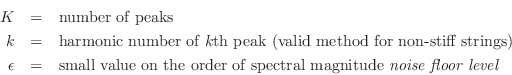
Since string spectra typically exhibit harmonically spaced nulls associated with the excitation and/or observation points, as well as from other phenomena such as recording multipath and/or reverberation, it is advisable to restrict to a range that does not include any spectral nulls (or simply omit index when $k{\hat f}_0$ is too close to a spectral null), since even one spectral null can push the product of peak amplitudes to a very small value. As a practical matter, it is important to inspect the magnitude spectra of the data manually to ensure that a robust row of peaks is being matched by the harmonic comb. For example, a display of the frame magnitude spectrum overlaid with vertical lines at the optimized harmonic-comb frequencies yields an effective picture of the F0 estimate in which typical problems (such as octave errors) are readily seen.

References on F0 Estimation

An often-cited book on classical methods for pitch detection, particularly for voice, is that by Hess [192]. The harmonic comb method can be considered an approximate maximum-likelihood pitch estimator, and more accurate maximum-likelihood methods have been worked out [114,547,376,377]. More recently, Klapuri has been developing some promising methods for multiple pitch estimation [254,253,252].^7.12A comparison of real-time pitch-tracking algorithms applied to guitar is given in [260], with consideration of latency (time delay).

Extension to Stiff Strings

An advantage of the harmonic-comb method, as well as other frequency-domain maximum-likelihood pitch-estimation methods, is that it is easily extended to accommodate stiff strings. For this, the stretch-factor in the spectral-peak center-frequencies can be estimated--the so-called coefficient of inharmonicity, and then the harmonic-comb (or other maximum-likelihood spectral-matching template) can be stretched by the same amount, so that when set to the correct pitch, the template matches the data spectrum more accurately than if harmonicity is assumed.

EDR-Based Loop-Filter Design

This section discusses use of the Energy Decay Relief (EDR) (§3.2.2) to measure the decay times of the partial overtones in a recorded vibrating string.

First we derive what to expect in the case of a simplified string model along the lines discussed in §6.7 above. Assume we have the synthesis model of Fig.6.12, where now the loss factor is replaced by the digital filter that we wish to design. Let $\underline{x}(n)$ denote the contents of the delay line as a vector at time , with $\underline{x}(0)$ denoting the initial contents of the delay line.

For simplicity, we define the EDR based on a length DFT of the delay-line vector $\underline{x}$ , and use a rectangular window with a ``hop size'' of samples, i.e.,

$\displaystyle \underline{X}_m(\omega_k) \isdef \dft _{N,\omega_k}\{\underline{x}_m\}, \quad m=0,1,2,\ldots,$

where $\underline{x}_m(n)\isdef \underline{x}(mN)$ . That is $\underline{x}_m$ is simply the

th successive snapshot of the delay-line contents, where the snapshots are taken once every

samples. We may interpret $\underline{X}_m$ as

th short-time spectrum of the output signal $y^{+}(n)$ shown in Fig.6.12. Due to the special structure of our synthesis model, we have

$\displaystyle \underline{X}_m(\omega_k) = H_l^m(\omega_k) \underline{X}_0(\omega_k)$

for each DFT bin number $k\in[0,N-1]$ .

Applying the definition of the EDR (§3.2.2) to this short-time spectrum gives

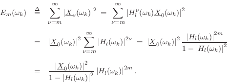
$\begin{eqnarray*} E_m(\omega_k) &\isdef & \sum_{\nu=m}^\infty \left\vert\underl... ...omega_k)\right\vert^2} \left\vert H_l(\omega_k)\right\vert^{2m}. \end{eqnarray*}$

We therefore have the following recursion for successive EDR time-slices:^7.13

$\displaystyle E_{m+1}(\omega_k) = \left\vert H_l(\omega_k)\right\vert^2 E_m(\omega_k)$

Since we normally try to fit straight-line decays to the EDR on a log scale (typically a decibel scale), we will see the relation

$\displaystyle \log(E_{m+1}) = \log(E_m) + \log(\vert H_l\vert^2),$

where the common argument $\omega_k$ is dropped for notational simplicity. Since we require $\vert H_l(\omega_k)\vert<1$ for stability of the filtered-delay loop, the EDR decays monotonically in this example. Thus, the measured slope of the partial overtone decays will be found to be proportional to $\log(\vert H_l\vert)$ .

This analysis can be generalized to a time-varying model in which the loop filter is allowed to change once per ``period'' .^7.14

An online laboratory exercise covering the practical details of measuring overtone decay-times and designing a corresponding loop filter is given in [280].

Next Section:
String Coupling Effects
Previous Section:
The Externally Excited String