Comb filters get their name from the ``comb-like'' appearance of their
amplitude response (gain versus frequency), as shown in
Figures 2.25, 2.26, and 2.27.
For a review of frequency-domain analysis
of digital filters, see, e.g., [449].
Figure:
Amplitude responses of the
feed forward comb-filter
 (diagrammed in Fig.2.23) with
  and
and  ,
,  , and
, and  .
a) Linear amplitude scale. b) Decibel scale. The frequency axis goes
from 0 to the sampling rate (instead of only half the
sampling rate, which is more typical for real filters) in order to
display the fact that the number of notches is exactly (as
opposed to ``
.
a) Linear amplitude scale. b) Decibel scale. The frequency axis goes
from 0 to the sampling rate (instead of only half the
sampling rate, which is more typical for real filters) in order to
display the fact that the number of notches is exactly (as
opposed to `` '').
'').
![\includegraphics[width=\twidth ]{eps/ffcfar}](http://www.dsprelated.com/josimages_new/pasp/img499.png) |
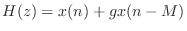
The transfer function of the feedforward comb filter Eq. (2.2) is
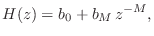 |
(3.3) |
so that the amplitude response (gain versus frequency) is
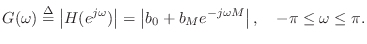 |
(3.4) |
This is plotted in Fig.
2.25 for
,

, and

,
, and
.
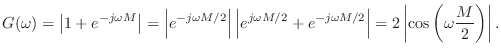
When

, we get the simplified result
In this case, we obtain
 nulls
nulls, which are points
(frequencies) of zero gain in the amplitude response. Note that in
flangers, these nulls are
moved slowly over time by
modulating the delay length
. Doing this smoothly requires
interpolated delay lines (see Chapter
4 and
Chapter
5).
Next Section: Feedback
Comb Filter Amplitude ResponsePrevious Section: Feedback Comb Filters