


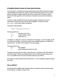
A Simplified Matlab Function for Power Spectral Density
In an earlier post, I showed how to compute power spectral density (PSD) of a discrete-time signal using the Matlab function pwelch. Pwelch is a useful function because it gives the correct output, and it has the option to average multiple Discrete Fourier Transforms (DFTs). However, a typical function call has five arguments, and it can be hard to remember how to set them all and how they default.
In this post, I create a simplified PSD function by putting a wrapper on pwelch that sets some parameters and converts the output units from W/Hz to dBW/bin. The function is named psd_simple.m, and its code is listed in the appendix.
Fractional Delay FIR Filters
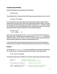
Consider the following Finite Impulse Response (FIR) coefficients:
b = [b0 b1 b2 b1 b0]
These coefficients form a 5-tap symmetrical FIR filter having constant group delay [1,2] over 0 to fs/2 of:
D = (ntaps - 1)/2 = 2 samples
For a symmetrical filter with an odd number of taps, the group delay is always an integer number of samples, while for one with an even number of taps, the group delay is always an integer + 0.5 samples. Can we design a filter with arbitrary delay, say 9.3 samples? The answer is yes -- It is possible to design a non-symmetrical FIR filter with arbitrary group delay which is approximately constant over a wide band, with approximately flat magnitude response [3,4]. Let the desired group delay be:
D = (ntaps - 1)/2 + u
= D0 + u samples, (1)
where we call u the fractional delay and -0.5 <= u <= 0.5. D0 is the fixed portion of the total delay; it is determined by ntaps. The appendix lists a simple Matlab function frac_delay_fir.m to compute FIR coefficients for a given value of u and ntaps. The function provides coefficients with approximately flat delay and frequency responses over a frequency range approaching 0 to fs/2.
In this post, we'll present a couple of examples using the function, then discuss the theory behind it. Finally, we'll look at an example of a fractional delay lowpass FIR filter with arbitrary cut-off frequency.
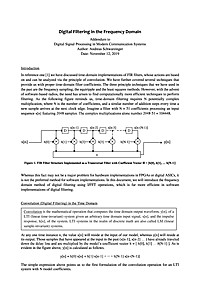
Digital Filtering in the Frequency Domain
Time domain digital filtering, whether implemented using FIR or IIR techniques, has been very well documented in literature and been thoroughly used in many base band processor designs. However, with the advent of software defined radios as well as CPU support in more recent baseband processors, it has become possible and often desirable to filter signals in software rather than digital hardware. Whereas, time domain digital filtering can certainly be implemented in software as well, it becomes highly inefficient as the number of filter taps grows. Frequency domain filtering, using FFT and IFFT operations, is significantly more efficient and surprisingly easy to understand. This document introduces the reader to frequency domain filtering both in theory and in practice via a MatLab script.
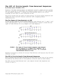
The DFT of Finite-Length Time-Reversed Sequences
Recently I've been reading papers on underwater acoustic communications systems and this caused me to investigate the frequency-domain effects of time-reversal of time-domain sequences. I created this article because there is so little coverage of this topic in the literature of DSP.
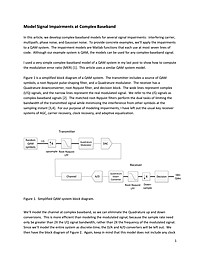
Model Signal Impairments at Complex Baseband
In this article, we develop complex-baseband models for several signal impairments: interfering carrier, multipath, phase noise, and Gaussian noise. To provide concrete examples, we'll apply the impairments to a QAM system. The impairment models are Matlab functions that each use at most seven lines of code. Although our example system is QAM, the models can be used for any complex-baseband signal.
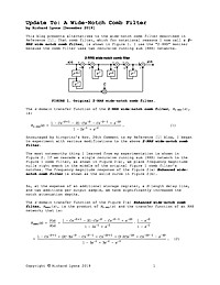
Update To: A Wide-Notch Comb Filter
This article presents alternatives to the wide-notch comb filter described in Reference [1].
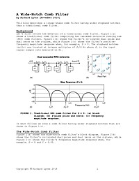
A Wide-Notch Comb Filter
This article describes a linear-phase comb filter having wider stopband notches than a traditional comb filter.
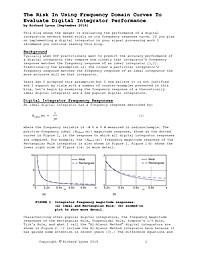
The Risk In Using Frequency Domain Curves To Evaluate Digital Integrator Performance
This article shows the danger in evaluating the performance of a digital integration network based solely on its frequency response curve. If you plan on implementing a digital integrator in your signal processing work I recommend you continue reading this article.
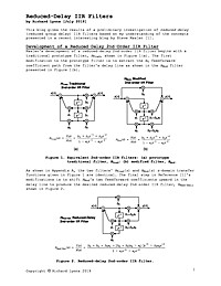
Reduced-Delay IIR Filters
This document describes a straightforward method to significantly reduce the number of necessary multiplies per input sample of traditional IIR lowpass and highpass digital filters.

A Quadrature Signals Tutorial: Complex, But Not Complicated
Quadrature signals are based on the notion of complex numbers and perhaps no other topic causes more heartache for newcomers to DSP than these numbers and their strange terminology of j operator, complex, imaginary, real, and orthogonal. If you're a little unsure of the physical meaning of complex numbers and the j = √-1 operator, don't feel bad because you're in good company. Why even Karl Gauss, one the world's greatest mathematicians, called the j operator the "shadow of shadows". Here we'll shine some light on that shadow so you'll never have to call the Quadrature Signal Psychic Hotline for help. Quadrature signal processing is used in many fields of science and engineering, and quadrature signals are necessary to describe the processing and implementation that takes place in modern digital communications systems. In this tutorial we'll review the fundamentals of complex numbers and get comfortable with how they're used to represent quadrature signals. Next we examine the notion of negative frequency as it relates to quadrature signal algebraic notation, and learn to speak the language of quadrature processing. In addition, we'll use three-dimensional time and frequency-domain plots to give some physical meaning to quadrature signals. This tutorial concludes with a brief look at how a quadrature signal can be generated by means of quadrature-sampling.
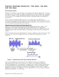
Digital Envelope Detection: The Good, the Bad, and the Ugly
Recently I've been thinking about the process of envelope detection. Tutorial information on this topic is readily available but that information is spread out over a number of DSP textbooks and many Internet web sites. The purpose of this blog is to summarize various digital envelope detection methods in one place. Here I focus of envelope detection as it is applied to an amplitude-fluctuating sinusoidal signal where the positive-amplitude fluctuations (the sinusoid's envelope) contain some sort of information. Let's begin by looking at the simplest envelope detection method.
Introduction of C Programming for DSP Applications
Appendix C of the book : Real-Time Digital Signal Processing: Implementations, Application and Experiments with the TMS320C55X
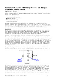
Understanding the 'Phasing Method' of Single Sideband Demodulation
There are four ways to demodulate a transmitted single sideband (SSB) signal. Those four methods are: synchronous detection, phasing method, Weaver method, and filtering method. Here we review synchronous detection in preparation for explaining, in detail, how the phasing method works. This blog contains lots of preliminary information, so if you're already familiar with SSB signals you might want to scroll down to the 'SSB DEMODULATION BY SYNCHRONOUS DETECTION' section.
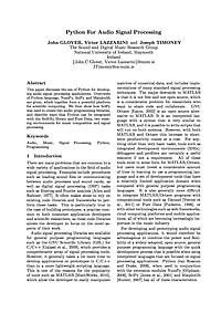
Python For Audio Signal Processing
This paper discusses the use of Python for developing audio signal processing applications. Overviews of Python language, NumPy, SciPy and Matplotlib are given, which together form a powerful platform for scientific computing. We then show how SciPy was used to create two audio programming libraries, and describe ways that Python can be integrated with the SndObj library and Pure Data, two existing environments for music composition and signal processing.
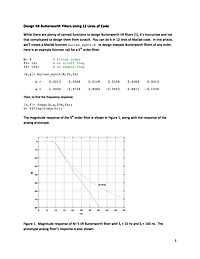
Design IIR Butterworth Filters Using 12 Lines of Code
While there are plenty of canned functions to design Butterworth IIR filters [1], it's instructive and not that complicated to design them from scratch. You can do it in 12 lines of Matlab code.
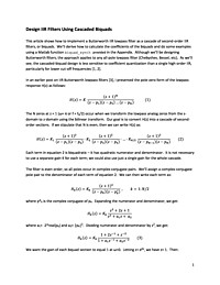
Design IIR Filters Using Cascaded Biquads
This article shows how to implement a Butterworth IIR lowpass filter as a cascade of second-order IIR filters, or biquads. We'll derive how to calculate the coefficients of the biquads and do some examples using a Matlab function biquad_synth provided in the Appendix. Although we'll be designing Butterworth filters, the approach applies to any all-pole lowpass filter (Chebyshev, Bessel, etc). As we'll see, the cascaded-biquad design is less sensitive to coefficient quantization than a single high-order IIR, particularly for lower cut-off frequencies.
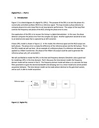
Digital PLL's -- Part 1
We will use Matlab to model the DPLL in the time and frequency domains (Simulink is also a good tool for modeling a DPLL in the time domain). Part 1 discusses the time domain model; the frequency domain model will be covered in Part 2. The frequency domain model will allow us to calculate the loop filter parameters to give the desired bandwidth and damping, but it is a linear model and cannot predict acquisition behavior. The time domain model can be made almost identical to the gate-level system, and as such, is able to model acquisition.
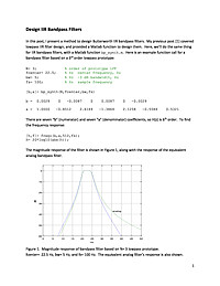
Design IIR Bandpass Filters
In this post, I present a method to design Butterworth IIR bandpass filters. My previous post [1] covered lowpass IIR filter design, and provided a Matlab function to design them. Here, we'll do the same thing for IIR bandpass filters, with a Matlab function bp_synth.m


