


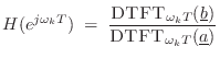
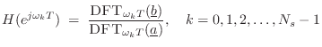
Frequency Response as a Ratio of DTFTs
From Eq.![]() (6.5), we have
(6.5), we have
![]() , so that the
frequency response is
, so that the
frequency response is
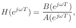
where
![\begin{eqnarray*}
{\underline{b}}&\isdef & [b_0,b_1,\ldots,b_M,0,\ldots]\\
{\underline{a}}&\isdef & [1,a_1,\ldots,a_N,0,\ldots],
\end{eqnarray*}](http://www.dsprelated.com/josimages_new/filters/img855.png)
and the DTFT is as defined in Eq.![]() (7.1).
(7.1).
From the above relations, we may express the frequency response of any IIR filter as a ratio of two finite DTFTs:
This expression provides a convenient basis for the computation of an IIR frequency response in software, as we pursue further in the next section.
Frequency Response in Matlab
In practice, we usually work with a sampled frequency axis. That
is, instead of evaluating the transfer function
![]() at
at
![]() to obtain the frequency response
to obtain the frequency response
![]() , where
, where ![]() is continuous radian frequency, we compute instead
is continuous radian frequency, we compute instead
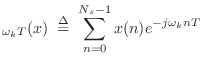
To avoid undersampling
![]() , we must have
, we must have ![]() , and to
avoid undersampling
, and to
avoid undersampling
![]() , we must have
, we must have ![]() . In general,
. In general,
![]() will be undersampled (when
will be undersampled (when ![]() ), because it is the
quotient of
), because it is the
quotient of
![]() over
over
![]() . This means, for example, that
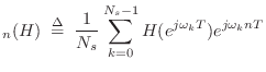
computing the impulse response
. This means, for example, that
computing the impulse response ![]() from the sampled frequency
response
from the sampled frequency
response
![]() will be time aliased in general. I.e.,
will be time aliased in general. I.e.,
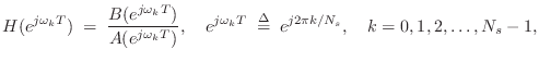
As is well known, when the DFT length ![]() is a power of 2, e.g.,
is a power of 2, e.g.,
![]() , the DFT can be computed extremely efficiently using
the Fast Fourier Transform (FFT). Figure 7.1 gives an
example matlab script for computing the frequency response of an IIR
digital filter using two FFTs. The Matlab function freqz
also uses this method when possible (e.g., when
, the DFT can be computed extremely efficiently using
the Fast Fourier Transform (FFT). Figure 7.1 gives an
example matlab script for computing the frequency response of an IIR
digital filter using two FFTs. The Matlab function freqz
also uses this method when possible (e.g., when ![]() is a power of 2).
is a power of 2).
function [H,w] = myfreqz(B,A,N,whole,fs) %MYFREQZ Frequency response of IIR filter B(z)/A(z). % N = number of uniform frequency-samples desired % H = returned frequency-response samples (length N) % w = frequency axis for H (length N) in radians/sec % Compatible with simple usages of FREQZ in Matlab. % FREQZ(B,A,N,whole) uses N points around the whole % unit circle, where 'whole' is any nonzero value. % If whole=0, points go from theta=0 to pi*(N-1)/N. % FREQZ(B,A,N,whole,fs) sets the assumed sampling % rate to fs Hz instead of the default value of 1. % If there are no output arguments, the amplitude and % phase responses are displayed. Poles cannot be % on the unit circle. A = A(:).'; na = length(A); % normalize to row vectors B = B(:).'; nb = length(B); if nargin < 3, N = 1024; end if nargin < 4, if isreal(b) & isreal(a), whole=0; else whole=1; end; end if nargin < 5, fs = 1; end Nf = 2*N; if whole, Nf = N; end w = (2*pi*fs*(0:Nf-1)/Nf)'; H = fft([B zeros(1,Nf-nb)]) ./ fft([A zeros(1,Nf-na)]); if whole==0, w = w(1:N); H = H(1:N); end if nargout==0 % Display frequency response if fs==1, flab = 'Frequency (cyles/sample)'; else, flab = 'Frequency (Hz)'; end subplot(2,1,1); % In octave, labels go before plot: plot([0:N-1]*fs/N,20*log10(abs(H)),'-k'); grid('on'); xlabel(flab'); ylabel('Magnitude (dB)'); subplot(2,1,2); plot([0:N-1]*fs/N,angle(H),'-k'); grid('on'); xlabel(flab); ylabel('Phase'); end |
Example LPF Frequency Response Using freqz
Figure 7.2 lists a short matlab program illustrating usage of freqz in Octave (as found in the octave-forge package). The same code should also run in Matlab, provided the Signal Processing Toolbox is available. The lines of code not pertaining to plots are the following:
  [B,A] = ellip(4,1,20,0.5); % Design lowpass filter B(z)/A(z)
  [H,w] = freqz(B,A);        % Compute frequency response H(w)
The filter example is a recursive fourth-order elliptic function lowpass filter cutting off at half the Nyquist limit (``
  plot(w,abs(H));
  plot(w,angle(H));
However, the example of Fig.7.2 uses more detailed ``compatibility'' functions listed in Appendix J. In particular, the freqplot utility is a simple compatibility wrapper for plot with label and title support (see §J.2 for Octave and Matlab version listings), and saveplot is a trivial compatibility wrapper for the print function, which saves the current plot to a disk file (§J.3). The saved freqplot plots are shown in Fig.7.3(a) and Fig.7.3(b).8.3
[B,A] = ellip(4,1,20,0.5); % Design the lowpass filter [H,w] = freqz(B,A); % Compute its frequency response % Plot the frequency response H(w): % figure(1); freqplot(w,abs(H),'-k','Amplitude Response',... 'Frequency (rad/sample)', 'Gain'); saveplot('../eps/freqzdemo1.eps'); figure(2); freqplot(w,angle(H),'-k','Phase Response',... 'Frequency (rad/sample)', 'Phase (rad)'); saveplot('../eps/freqzdemo2.eps'); % Plot frequency response in a "multiplot" like Matlab uses: % figure(3); plotfr(H,w/(2*pi)); if exist('OCTAVE_VERSION') disp('Cannot save multiplots to disk in Octave') else saveplot('../eps/freqzdemo3.eps'); end |
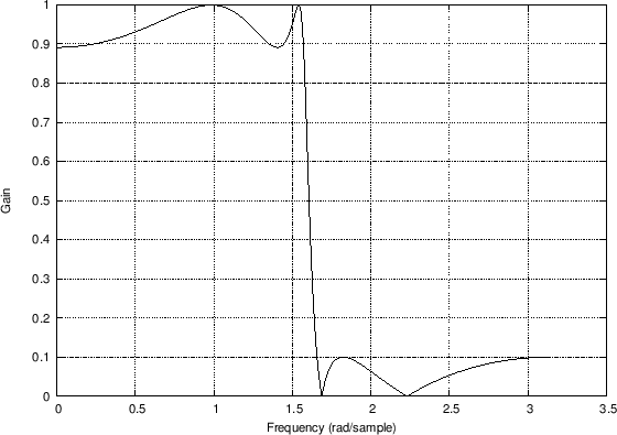
Amplitude
Response 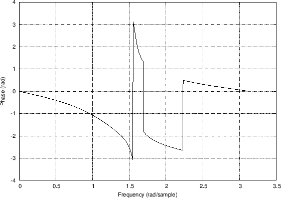
Phase Response |
Next Section:
Phase and Group Delay
Previous Section:
Polar Form of the Frequency Response


