


Matlab Utilities
This appendix provides software listings for various analysis utilities written in matlab. Except for plot-related commands, they should be compatible either Matlab or Octave.
Time Plots: myplot.m
function myplot(x, y, sym, ttl, xlab, ylab, grd, lgnd)
% MYPLOT - Generic plot - compatibility wrapper for plot()
%          Octave version.  See below for Matlab version.
%          In Octave, title and axis labels must be issued
%          BEFORE the plot() command.

  if nargin<8, lgnd=''; end
  if nargin<7, grd=1; end
  if nargin<6, ylab=''; end
  if nargin<5, xlab=''; end
  if nargin<4, ttl=''; end
  if nargin<3, sym='*k'; end
  if nargin<2, y=x; x=0:length(y)-1; end

  title(ttl);
  ylabel(ylab);
  xlabel(xlab);
  if grd, grid('on'); else grid('off'); end
  plot(x,y,sym);
  legend(lgnd);
|
function myplot(x, y, sym, ttl, xlab, ylab, grd, lgnd)
% MYPLOT - Generic plot - compatibility wrapper for plot()
%          Matlab version. Title and axis labels must be
%          placed AFTER the plot() command.

  if nargin<8, lgnd=''; end
  if nargin<7, grd=1; end
  if nargin<6, ylab=''; end
  if nargin<5, xlab=''; end
  if nargin<4, ttl=''; end
  if nargin<3, sym='*k'; end
  if nargin<2, y=x; x=0:length(y)-1; end

  plot(x,y,sym);
  title(ttl);
  ylabel(ylab);
  xlabel(xlab);
  if grd, grid('on'); end
  legend(lgnd);
|
Frequency Plots: freqplot.m
function freqplot(fdata, ydata, symbol, ttl, xlab, ylab)
% FREQPLOT - Plot a function of frequency:
%
%   freqplot(fdata[,ydata[,symbol[,title[,xlab[,ylab]]]]])
%
%   This version is most compatible with Octave.
%   In Matlab, the title and axis labels may be lost.
%   For Matlab compatibility, move the plot() command
%   before title() and axis label commands.

  if nargin<6, ylab=''; end
  if nargin<5, xlab='Frequency'; end
  if nargin<4, ttl=''; end
  if nargin<3, symbol=''; end
  if nargin<2, ydata=fdata; fdata=0:length(ydata)-1; end

  if ttl, title(ttl); end
  if length(ylab)>0, ylabel(ylab); end
  if length(xlab)>0, xlabel(xlab); end
  grid('on');
  plot(fdata,ydata,symbol);
|
function freqplot(fdata, ydata, symbol, ttl, xlab, ylab) % FREQPLOT - Plot a function of time, Matlab version. if nargin<6, ylab=''; end if nargin<5, xlab='Frequency (Hz)'; end if nargin<4, ttl=''; end if nargin<3, symbol=''; end if nargin<2, fdata=0:length(ydata)-1; end plot(fdata,ydata,symbol); grid; if ttl, title(ttl); end if ylab, ylabel(ylab); end xlabel(xlab); |
Saving Plots to Disk: saveplot.m
function saveplot(filename,optargs)
% SAVEPLOT - Save current plot to disk in a PostScript file.
%            This version is compatible only with Octave.
%            In Matlab, just say 'print -deps[c] filename'.
%            *** MULTIPLOT MODE NOT SUPPORTED ***
%            (only get last plot)

if (nargin<2), optargs = ''; end;
% optargs to consider:
%   landscape
%   color
%   solid
%   "<fontname>" <fontsize>
%   lw <width> [default = 1.0]

gset terminal push

gset nomultiplot % can't set out terminal in multiplot mode
%gset terminal fig % in this output format, you can edit it!
cmd=['gset terminal postscript eps monochrome enhanced',...
     optargs];
eval(cmd);

disp(sprintf('Writing current plot to %s',filename));
cmd = sprintf('gset output \'%s\';',filename); eval(cmd);

replot
% remultiplot -- does not yet exist in gnuplot
closeplot

gset terminal pop
|
function saveplot(filename) % SAVEPLOT - Save current plot to disk in a PostScript file. % This version is compatible only with Matlab. cmd = ['print -deps ',filename]; % for color, use '-depsc' disp(cmd); eval(cmd); |
Frequency Response Plots: plotfr.m
Figure J.7 lists a Matlab function for plotting frequency-response magnitude and phase. (See also Fig.7.1.) Since Octave does not yet support saving multiple ``subplots'' to disk for later printing, we do not have an Octave-compatible version here. At present, Matlab's graphics support is much more extensive and robust than that in Octave's (which is based on a shaky and Matlab-incompatible interface to gnuplot). Another free alternative to consider for making nice Matlab-style 2D plots is matplotlib.
function [plothandle] = plotfr(X,f); % PLOTFR - Plot frequency-response magnitude & phase. % Requires Mathworks Matlab. % % X = frequency response % f = vector of corresponding frequency values Xm = abs(X); % Amplitude response Xmdb = 20*log10(Xm); % Prefer dB for audio work Xp = angle(X); % Phase response if nargin<2, N=length(X); f=(0:N-1)/(2*(N-1)); end subplot(2,1,1); plot(f,Xmdb,'-k'); grid; ylabel('Gain (dB)'); xlabel('Normalized Frequency (cycles/sample)'); axis tight; text(-0.07,max(Xmdb),'(a)'); subplot(2,1,2); plot(f,Xp,'-k'); grid; ylabel('Phase Shift (radians)'); xlabel('Normalized Frequency (cycles/sample)'); axis tight; text(-0.07,max(Xp),'(b)'); if exist('OCTAVE_VERSION') plothandle = 0; % gcf undefined in Octave else plothandle = gcf; end |
Partial Fraction Expansion: residuez.m
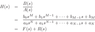
Figure J.8 gives a listing of a matlab function for computing
a ``left-justified'' partial fraction expansion (PFE) of an IIR
digital filter
![]() as described in §6.8 (and
below). This function, along with its ``right justified''
counterpart, residued, are included in the
octave-forge matlab library for Octave.J.1
as described in §6.8 (and
below). This function, along with its ``right justified''
counterpart, residued, are included in the
octave-forge matlab library for Octave.J.1
function [r, p, f, m] = residuez(B, A, tol) if nargin<3, tol=0.001; end NUM = B(:)'; DEN = A(:)'; % Matlab's residue does not return m (implied by p): [r,p,f,m]=residue(conj(fliplr(NUM)),conj(fliplr(DEN)),tol); p = 1 ./ p; r = r .* ((-p) .^m); if f, f = conj(fliplr(f)); end |
This code was written for Octave, but it also runs in Matlab if the 'm' outputs (pole multiplicity counts) are omitted (two places). The input arguments are compatible with the existing residuez function in the Matlab Signal Processing Toolbox.
Method
As can be seen from the code listing, this implementation of
residuez simply calls residue, which was written to
carry out the partial fraction expansions of ![]() -plane
(continuous-time) transfer functions
-plane
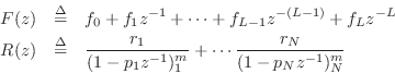
(continuous-time) transfer functions ![]() :
:
where ![]() is the ``quotient'' and
is the ``quotient'' and ![]() is the ``remainder'' in the PFE:
is the ``remainder'' in the PFE:
where
In the discrete-time case, we have the ![]() -plane transfer function
-plane transfer function
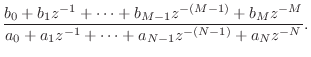
For compatibility with Matlab's residuez, we need a PFE of the form
where ![]() .
.
We see that the ![]() -plane case formally does what we desire if we
treat
-plane case formally does what we desire if we
treat ![]() -plane polynomials as polynomials in
-plane polynomials as polynomials in ![]() instead of
instead of
![]() . From Eq.
. From Eq.![]() (J.2), we see that this requires reversing the
coefficient-order of B and A in the call to
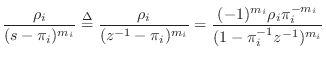
residue. In the returned result, we obtain terms such as
(J.2), we see that this requires reversing the
coefficient-order of B and A in the call to
residue. In the returned result, we obtain terms such as
Example with Repeated Poles
The following Matlab code performs a partial fraction expansion of a filter having three pairs of repeated roots (one real and two complex):J.2
N = 1000;  % number of time samples to compute
A = [ 1 0 0 1 0 0 0.25];
B = [ 1 0 0 0 0 0 0];

% Compute "trusted" impulse response:
h_tdl = filter(B, A, [1 zeros(1, N-1)]);

% Compute partial fraction expansion (PFE):
[R,P,K] = residuez(B, A);

% PFE impulse response:
n = [0:N-1];
h_pfe = zeros(1,N);
for i = 1:size(R)
  % repeated roots are not detected exactly:
  if i>1 && abs(P(i)-P(i-1))<1E-7
    h_pfe = h_pfe + (R(i) * (n+1) .* P(i).^n);
    disp(sprintf('Pole %d is a repeat of pole %d',i,i-1));
    % if i>2 && abs(P(i)-P(i-2))<1E-7 ...
  else
    h_pfe = h_pfe + (R(i) * P(i).^n);
  end
end

err = abs(max(h_pfe-h_tdl)) % should be about 5E-8
Partial Fraction Expansion: residued.m
Figure J.9 gives a listing of a matlab function for computing a
``right justified'' partial fraction expansion (PFE) of an IIR digital
filter
![]() as described in §6.8 (and below).
as described in §6.8 (and below).
The code in Fig.J.9 was written to work in Octave, and also in Matlab if the 'm' argument is omitted (in two places).
function [r, p, f, e] = residued(b, a, toler) if nargin<3, toler=0.001; end NUM = b(:)'; DEN = a(:)'; nb = length(NUM); na = length(DEN); f = []; if na<=nb f = filter(NUM,DEN,[1,zeros(nb-na)]); NUM = NUM - conv(DEN,f); NUM = NUM(nb-na+2:end); end [r,p,f2,e] = residuez(NUM,DEN,toler); |
Method
The FIR part is first extracted, and the (strictly proper) remainder
is passed to residuez for expansion of the IIR part (into a
sum of complex resonators). One must remember that, in this case, the
impulse-response of the IIR part ![]() begins after the
impulse-response of the FIR part
begins after the
impulse-response of the FIR part ![]() has finished, i.e.,
has finished, i.e.,
See §6.8.8 for an example usage of residued (with a comparison to residuez).
Parallel SOS to Transfer Function: psos2tf.m
Figure J.10 lists a matlab function for computing the direct-form
transfer-function polynomials ![]() from parallel
second-order section coefficients. This is in contrast to the
existing function sos2tf which converts series
second-order sections to transfer-function form.
from parallel
second-order section coefficients. This is in contrast to the
existing function sos2tf which converts series
second-order sections to transfer-function form.
function [B,A] = psos2tf(sos,g) if nargin<2, g=1; end [nsecs,tmp] = size(sos); if nsecs<1, B=[]; A=[]; return; end Bs = sos(:,1:3); As = sos(:,4:6); B = Bs(1,:); A = As(1,:); for i=2:nsecs B = conv(B,As(i,:)) + conv(A,Bs(i,:)); A = conv(A,As(i,:)); end |
Group Delay Computation: grpdelay.m
Figure J.11 gives a listing of a matlab program for computing
the group delay of an IIR digital filter
![]() using the
method described in §7.6.6.
using the
method described in §7.6.6.
In Matlab with the Signal Processing Toolbox installed, (or Octave with the Octave Forge package installed), say 'help grpdelay' for usage documentation, and say 'type grpdelay' to additionally see test, demo, and plotting code. Here, we include only the code relevant to computation of the group delay itself.
function [gd,w] = grpdelay(b,a,nfft,whole,Fs)

  if (nargin<1 || nargin>5)
    usage("[g,w]=grpdelay(b [, a [, n [,'whole'[,Fs]]]])");
  end
  if nargin<5
    Fs=0; % return w in radians per sample
    if nargin<4, whole='';
    elseif ~isstr(whole)
      Fs = whole;
      whole = '';
    end
    if nargin<3, nfft=512; end
    if nargin<2, a=1; end
  end

  if strcmp(whole,'whole')==0, nfft = 2*nfft; end

  w = 2*pi*[0:nfft-1]/nfft;
  if Fs>0, w = Fs*w/(2*pi); end

  oa = length(a)-1;             % order of a(z)
  oc = oa + length(b)-1;        % order of c(z)
  c = conv(b,fliplr(a));	% c(z) = b(z)*a(1/z)*z^(-oa)
  cr = c.*[0:oc];               % derivative of c wrt 1/z
  num = fft(cr,nfft);
  den = fft(c,nfft);
  minmag = 10*eps;
  polebins = find(abs(den)<minmag);
  for b=polebins
    disp('*** grpdelay: group delay singular! setting to 0')
    num(b) = 0;
    den(b) = 1;
  end
  gd = real(num ./ den) - oa;

  if strcmp(whole,'whole')==0
    ns = nfft/2; % Matlab convention - should be nfft/2 + 1
    gd = gd(1:ns);
    w = w(1:ns);
  end

  w = w'; % Matlab returns column vectors
  gd = gd';
|
Matlab listing: fold.m
The fold() function ``time-aliases'' the noncausal part of a function onto its causal part. When applied to the inverse Fourier transform of a log-spectrum, it converts non-minimum-phase zeros to minimum-phase zeros. (See §J.11 for an example usage.)
function [rw] = fold(r) % [rw] = fold(r) % Fold left wing of vector in "FFT buffer format" % onto right wing % J.O. Smith, 1982-2002 [m,n] = size(r); if m*n ~= m+n-1 error('fold.m: input must be a vector'); end flipped = 0; if (m > n) n = m; r = r.'; flipped = 1; end if n < 3, rw = r; return; elseif mod(n,2)==1, nt = (n+1)/2; rw = [ r(1), r(2:nt) + conj(r(n:-1:nt+1)), ... 0*ones(1,n-nt) ]; else nt = n/2; rf = [r(2:nt),0]; rf = rf + conj(r(n:-1:nt+1)); rw = [ r(1) , rf , 0*ones(1,n-nt-1) ]; end; if flipped rw = rw.'; end |
Matlab listing: clipdb.m
The clipdb() function prevents the log magnitude of a signal from being too large and negative. (See §J.11 for an example usage.)
function [clipped] = clipdb(s,cutoff)
% [clipped] = clipdb(s,cutoff)
% Clip magnitude of s at its maximum + cutoff in dB.
% Example: clip(s,-100) makes sure the minimum magnitude
% of s is not more than 100dB below its maximum magnitude.
% If s is zero, nothing is done.

clipped = s;
as = abs(s);
mas = max(as(:));
if mas==0, return; end
if cutoff >= 0, return; end
thresh = mas*10^(cutoff/20); % db to linear
toosmall = find(as < thresh);
clipped = s;
clipped(toosmall) = thresh;
Matlab listing: mps.m and test program
This section lists and describes the Matlab/Octave function mps which estimates a minimum-phase spectrum given only the spectral magnitude. A test program for mps together with a listing of its output are given in §J.11 below. See §11.7 for related discussion.
Matlab listing: mps.m
function [sm] = mps(s)
% [sm] = mps(s)
% create minimum-phase spectrum sm from complex spectrum s
   sm = exp( fft( fold( ifft( log( clipdb(s,-100) )))));
The clipdb and fold utilities are listed and described in §J.10 and §J.9, respectively.
Note that mps.m must be given a whole spectrum in ``FFT buffer format''. That is, it must contain dc and positive-frequency values followed by negative frequency values and be a power of 2 in length.
The mps function works well as long as the desired frequency
response is smooth. If there are any zeros on the frequency
axis (``notches''), the corresponding minimum-phase impulse response
will be time aliased because the corresponding exponentials in
the cepstrum never decay. To suppress time-aliasing to some extent,
the desired frequency response magnitude is clipped to 100 dB below
its maximum. Time aliasing can be reduced by interpolating the
desired frequency response s to a higher sampling density
(thereby increasing the time available for exponential decay in the
cepstral domain). However, for pure notches (zeros right on the unit
circle), no amount of oversampling will eliminate the time aliasing
completely. To avoid time aliasing in the cepstrum, such a desired
spectrum must be smoothed before taking the log and inverse
FFT. Zero-phase smoothing of the spectral magnitude is a typical
choice for this purpose. When greater accuracy is required, all notch
frequencies can be estimated so that terms of the form
![]() can be effectively ``divided out'' of the
desired spectrum and carried along as separate factors.
can be effectively ``divided out'' of the
desired spectrum and carried along as separate factors.
Matlab listing: tmps.m
Below is the test script (for ease of copy/paste extraction for online viewers). Following is the test script along with its output.
Note that this is a toy example intended only for checking the code on a simple example, and to illustrate how a spectrum gets passed in. In particular, the would-be minimum-phase impulse response computed by this example is clearly not even causal (thus indicating an insufficient spectral sampling density [FFT length]). Moreover, the starting spectrum (a sampled ideal lowpass-filter frequency response) has zeros on the unit circle, so there is no sampling density that is truly sufficient in the frequency domain (no sufficiently long FFT in the time domain).
spec = [1 1 1 0 0 0 1 1]'; % Lowpass cutting off at fs*3/8
format short;
mps(spec)
abs(mps(spec))
ifft(spec)
ifft(mps(spec))
Matlab diary: tmps.d
Below is the output of the test script with echo on in Matlab.
spec = [1 1 1 0 0 0 1 1]'; % Lowpass cutting off at fs*3/8
format short;
mps(spec)

ans =
   1.0000 - 0.0000i
   0.3696 - 0.9292i
  -0.2830 - 0.9591i
   0.0000 - 0.0000i
   0.0000 + 0.0000i
   0.0000 + 0.0000i
  -0.2830 + 0.9591i
   0.3696 + 0.9292i

abs(mps(spec))

ans =
    1.0000
    1.0000
    1.0000
    0.0000
    0.0000
    0.0000
    1.0000
    1.0000

ifft(spec)

ans =
   0.6250
   0.3018 - 0.0000i
  -0.1250
  -0.0518 - 0.0000i
   0.1250
  -0.0518 + 0.0000i
  -0.1250
   0.3018 + 0.0000i

ifft(mps(spec))

ans =
   0.1467 - 0.0000i
   0.5944 - 0.0000i
   0.4280 - 0.0000i
  -0.0159 - 0.0000i
  -0.0381 - 0.0000i
   0.1352 - 0.0000i
  -0.0366 - 0.0000i
  -0.2137 - 0.0000i
(The last four terms above would be zero if the result were causal.)
Signal Plots: swanalplot.m
Figure J.13 lists a Matlab script for plotting input and output signals for the simplest lowpass filter in §2.2, used in Fig.2.4 to produce Fig.2.5. This is not really a ``utility'' since it relies on global variables. It is instead a script containing mundane plotting code that was omitted from Fig.2.4 to make it fit on one page. I include it only because people keep asking for it! The script is compatible with Matlab only.
%swanalplot.m - plots needed by swanal.m

doplots = 1; % set to 0 to skip plots
dopause = 0; % set to 1 to pause after each plot
if doplots
  figure(gcf);
  subplot(2,1,1);
  ttl=sprintf('Filter Input Sinusoid, f(%d)=%0.2f',k,f(k));
  myplot(t,s,'*k',ttl);
  tinterp=0:(t(2)-t(1))/10:t(end); % interpolated time axis
  si = ampin*cos(2*pi*f(k)*tinterp+phasein); % for plot
  text(-1.5,0,'(a)');
  hold on; plot(tinterp,si,'--k'); hold off;
  subplot(2,1,2);
  ttl='Filter Output Sinusoid';
  myplot(t,y,'*k',ttl);
  text(-1.5,0,'(b)');
  if dopause, disp('PAUSING - [RETURN] to continue . . .');
  pause; end
  saveplot(sprintf('../eps/swanal-%d.eps',k));
end
|
Frequency Response Plot: swanalmainplot.m
Figure J.14 lists a Matlab script for plotting (in Fig.2.7) the overlay of the theoretical frequency response with that measured using simulated sine-wave analysis for the case of the simplest lowpass filter. It is written to run in the specific context of the matlab script listed in Fig.2.3 of §2.2. This is not a general-purpose ``utility'' because it relies on global variables defined in the calling script. This script is included only for completeness and is compatible with Matlab only.
% swanalmainplot.m % Compare measured and theoretical frequency response. % This script is invoked by swanalmainplot.m and family, % and requires context set up by the caller. figure(N+1); % figure number is arbitary subplot(2,1,1); ttl = 'Amplitude Response'; freqplot(f,gains,'*k',ttl,'Frequency (Hz)','Gain'); tar = 2*cos(pi*f/fs); % theoretical amplitude response hold on; freqplot(f,tar,'-k'); hold off; text(-0.08,mean(ylim),'(a)'); subplot(2,1,2); ttl = 'Phase Response'; tpr = -pi*f/fs; % theoretical phase response pscl = 1/(2*pi);% convert radian phase shift to cycles freqplot(f,tpr*pscl,'-k',ttl,'Frequency (cycles)',... 'Phase shift (cycles)'); hold on; freqplot(f,phases*pscl,'*k'); hold off; text(-0.08,mean(ylim),'(b)'); saveplot(plotfile); % set by caller |
Next Section:
Digital Filtering in Faust and PD
Previous Section:
Recursive Digital Filter Design


