


The Simplest Lowpass Filter
This chapter introduces analysis of digital filters applied to a very simple example filter. The initial treatment uses only high-school level math (trigonometry), followed by an easier but more advanced approach using complex variables. Several important topics in digital signal processing are introduced in an extremely simple setting, and motivation is given for the study of further topics such as complex variables and Fourier analysis [84].
Introduction
Musicians have been using filters for thousands of years to shape the sounds of their art in various ways. For example, the evolution of the physical dimensions of the violin constitutes an evolution in filter design. The choice of wood, the shape of the cutouts, the geometry of the bridge, and everything that affects resonance all have a bearing on how the violin body filters the signal induced at the bridge by the vibrating strings. Once a sound is airborne there is yet more filtering performed by the listening environment, by the pinnae of the ear, and by idiosyncrasies of the hearing process.
What is a Filter?
Any medium through which the music signal passes, whatever its form, can be regarded as a filter. However, we do not usually think of something as a filter unless it can modify the sound in some way. For example, speaker wire is not considered a filter, but the speaker is (unfortunately). The different vowel sounds in speech are produced primarily by changing the shape of the mouth cavity, which changes the resonances and hence the filtering characteristics of the vocal tract. The tone control circuit in an ordinary car radio is a filter, as are the bass, midrange, and treble boosts in a stereo preamplifier. Graphic equalizers, reverberators, echo devices, phase shifters, and speaker crossover networks are further examples of useful filters in audio. There are also examples of undesirable filtering, such as the uneven reinforcement of certain frequencies in a room with ``bad acoustics.'' A well-known signal processing wizard is said to have remarked, ``When you think about it, everything is a filter.''
A digital filter is just a filter that operates on digital signals, such as sound represented inside a computer. It is a computation which takes one sequence of numbers (the input signal) and produces a new sequence of numbers (the filtered output signal). The filters mentioned in the previous paragraph are not digital only because they operate on signals that are not digital. It is important to realize that a digital filter can do anything that a real-world filter can do. That is, all the filters alluded to above can be simulated to an arbitrary degree of precision digitally. Thus, a digital filter is only a formula for going from one digital signal to another. It may exist as an equation on paper, as a small loop in a computer subroutine, or as a handful of integrated circuit chips properly interconnected.
Why learn about filters?
Computer musicians nearly always use digital filters in every piece of music they create. Without digital reverberation, for example, it is difficult to get rich, full-bodied sound from the computer. However, reverberation is only a surface scratch on the capabilities of digital filters. A digital filter can arbitrarily shape the spectrum of a sound. Yet very few musicians are prepared to design the filter they need, even when they know exactly what they want in the way of a spectral modification. A goal of this book is to assist sound designers by listing the concepts and tools necessary for doing custom filter designs.
There is plenty of software available for designing digital filters [10,8,22]. In light of this available code, it is plausible to imagine that only basic programming skills are required to use digital filters. This is perhaps true for simple applications, but knowledge of how digital filters work will help at every phase of using such software.
Also, you must understand a program before you can modify it or extract pieces of it. Even in standard applications, effective use of a filter design program requires an understanding of the design parameters, which in turn requires some understanding of filter theory. Perhaps most important for composers who design their own sounds, a vast range of imaginative filtering possibilities is available to those who understand how filters affect sounds. In my practical experience, intimate knowledge of filter theory has proved to be a very valuable tool in the design of musical instruments. Typically, a simple yet unusual filter is needed rather than one of the classical designs obtainable using published software.
The Simplest Lowpass Filter
Let's start with a very basic example of the generic problem at hand: understanding the effect of a digital filter on the spectrum of a digital signal. The purpose of this example is to provide motivation for the general theory discussed in later chapters.
Our example is the simplest possible low-pass filter. A low-pass
filter is one which does not affect low frequencies and rejects high
frequencies. The function giving the gain of a filter at every
frequency is called the amplitude response (or magnitude
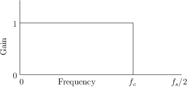
frequency response). The amplitude response of the ideal lowpass
filter is shown in Fig.1.1. Its gain is 1 in the
passband, which spans frequencies from 0 Hz to the cut-off
frequency ![]() Hz, and its gain is 0 in the stopband (all
frequencies above
Hz, and its gain is 0 in the stopband (all
frequencies above ![]() ). The output spectrum is obtained by
multiplying the input spectrum by the amplitude response of the
filter. In this way, signal components are eliminated (``stopped'')
at all frequencies above the cut-off frequency, while lower-frequency
components are ``passed'' unchanged to the output.
). The output spectrum is obtained by
multiplying the input spectrum by the amplitude response of the
filter. In this way, signal components are eliminated (``stopped'')
at all frequencies above the cut-off frequency, while lower-frequency
components are ``passed'' unchanged to the output.
Definition of the Simplest Low-Pass
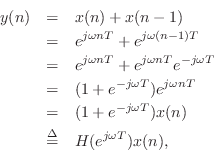
The simplest (and by no means ideal) low-pass filter is given by the following difference equation:
where

It is important when working with spectra to be able to convert time
from sample-numbers, as in Eq.![]() (1.1) above, to seconds. A more
``physical'' way of writing the filter equation is
(1.1) above, to seconds. A more
``physical'' way of writing the filter equation is
To further our appreciation of this example, let's write a computer
subroutine to implement Eq.![]() (1.1). In the computer,
(1.1). In the computer, ![]() and
and
![]() are data arrays and
are data arrays and ![]() is an array index. Since sound files
may be larger than what the computer can hold in memory all at
once, we typically process the data in blocks of some reasonable
size. Therefore, the complete filtering operation consists of two
loops, one within the other. The outer loop fills the input array
is an array index. Since sound files
may be larger than what the computer can hold in memory all at
once, we typically process the data in blocks of some reasonable
size. Therefore, the complete filtering operation consists of two
loops, one within the other. The outer loop fills the input array ![]() and empties the output array
and empties the output array ![]() , while the inner loop does the actual
filtering of the
, while the inner loop does the actual
filtering of the ![]() array to produce
array to produce ![]() . Let
. Let ![]() denote the block
size (i.e., the number of samples to be processed on each iteration of
the outer loop). In the C programming language, the inner loop
of the subroutine might appear as shown in Fig.1.3. The outer
loop might read something like ``fill
denote the block
size (i.e., the number of samples to be processed on each iteration of
the outer loop). In the C programming language, the inner loop
of the subroutine might appear as shown in Fig.1.3. The outer
loop might read something like ``fill ![]() from the input file,''
``call simplp,'' and ``write out
from the input file,''
``call simplp,'' and ``write out ![]() .''
.''
/* C function implementing the simplest lowpass:
 *
 *      y(n) = x(n) + x(n-1)
 *
 */
double simplp (double *x, double *y,
               int M, double xm1)
{
  int n;
  y[0] = x[0] + xm1;
  for (n=1; n < M ; n++) {
    y[n] =  x[n]  + x[n-1];
  }
  return x[M-1];
}
|
In this implementation, the first instance of ![]() is provided as
the procedure argument xm1. That way, both
is provided as
the procedure argument xm1. That way, both ![]() and
and ![]() can
have the same array bounds (
can
have the same array bounds (
![]() ). For convenience, the
value of xm1 appropriate for the next call to
simplp is returned as the procedure's value.
). For convenience, the
value of xm1 appropriate for the next call to
simplp is returned as the procedure's value.
We may call xm1 the filter's state. It is the current
``memory'' of the filter upon calling simplp. Since this
filter has only one sample of state, it is a first order
filter. When a filter is applied to successive blocks of a signal, it
is necessary to save the filter state after processing each block.
The filter state after processing block ![]() is then the starting state
for block
is then the starting state
for block ![]() .
.
Figure 1.4 illustrates a simple main program which calls simplp. The length 10 input signal x is processed in two blocks of length 5.
/* C main program for testing simplp */
main() {
  double x[10] = {1,2,3,4,5,6,7,8,9,10};
  double y[10];

  int i;
  int N=10;
  int M=N/2; /* block size */
  double xm1 = 0;

  xm1 = simplp(x, y, M, xm1);
  xm1 = simplp(&x[M], &y[M], M, xm1);

  for (i=0;i<N;i++) {
    printf("x[%d]=%f\ty[%d]=%f\n",i,x[i],i,y[i]);
  }
  exit(0);
}
/* Output:
 *    x[0]=1.000000     y[0]=1.000000
 *    x[1]=2.000000     y[1]=3.000000
 *    x[2]=3.000000     y[2]=5.000000
 *    x[3]=4.000000     y[3]=7.000000
 *    x[4]=5.000000     y[4]=9.000000
 *    x[5]=6.000000     y[5]=11.000000
 *    x[6]=7.000000     y[6]=13.000000
 *    x[7]=8.000000     y[7]=15.000000
 *    x[8]=9.000000     y[8]=17.000000
 *    x[9]=10.000000    y[9]=19.000000
 */
|
You might suspect that since Eq.![]() (1.1) is the simplest possible
low-pass filter, it is also somehow the worst possible low-pass
filter. How bad is it? In what sense is it bad? How do we even know it
is a low-pass at all? The answers to these and related questions will
become apparent when we find the frequency response of this
filter.
(1.1) is the simplest possible
low-pass filter, it is also somehow the worst possible low-pass
filter. How bad is it? In what sense is it bad? How do we even know it
is a low-pass at all? The answers to these and related questions will
become apparent when we find the frequency response of this
filter.
Finding the Frequency Response
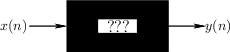
Think of the filter expressed by Eq.![]() (1.1) as a ``black box'' as
depicted in Fig.1.5. We want to know the effect of this black box
on the spectrum of
(1.1) as a ``black box'' as
depicted in Fig.1.5. We want to know the effect of this black box
on the spectrum of ![]() , where
, where ![]() represents the entire
input signal (see §A.1).
represents the entire
input signal (see §A.1).
Sine-Wave Analysis
Suppose we test the filter at each frequency separately. This is
called sine-wave analysis.2.1Fig.1.6 shows an example of
an input-output pair, for the filter of Eq.![]() (1.1), at the
frequency
(1.1), at the
frequency ![]() Hz, where
Hz, where ![]() denotes the sampling rate. (The
continuous-time waveform has been drawn through the samples for
clarity.) Figure 1.6a shows the input signal, and Fig.1.6b
shows the output signal.
denotes the sampling rate. (The
continuous-time waveform has been drawn through the samples for
clarity.) Figure 1.6a shows the input signal, and Fig.1.6b
shows the output signal.
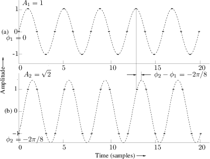 |
The ratio of the peak output amplitude to the peak input amplitude is
the filter gain at this frequency. From Fig.1.6 we find
that the gain is about 1.414 at the frequency ![]() . We may also
say the amplitude response is 1.414 at
. We may also
say the amplitude response is 1.414 at ![]() .
.
The phase of the output signal minus the phase of the input signal is
the phase response of the filter at this
frequency. Figure 1.6 shows that the filter of Eq.![]() (1.1) has a
phase response equal to
(1.1) has a
phase response equal to ![]() (minus one-eighth of a cycle) at the
frequency
(minus one-eighth of a cycle) at the
frequency ![]() .
.
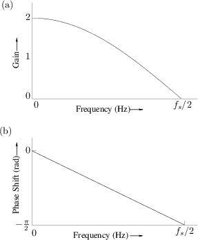
Continuing in this way, we can input a sinusoid at each frequency
(from 0 to ![]() Hz), examine the input and output waveforms as in
Fig.1.6, and record on a graph the peak-amplitude ratio (gain)
and phase shift for each frequency. The resultant pair of plots, shown
in Fig.1.7, is called the frequency response. Note that
Fig.1.6 specifies the middle point of each graph in Fig.1.7.
Hz), examine the input and output waveforms as in
Fig.1.6, and record on a graph the peak-amplitude ratio (gain)
and phase shift for each frequency. The resultant pair of plots, shown
in Fig.1.7, is called the frequency response. Note that
Fig.1.6 specifies the middle point of each graph in Fig.1.7.
Not every black box has a frequency response, however. What good is a pair of graphs such as shown in Fig.1.7 if, for all input sinusoids, the output is 60 Hz hum? What if the output is not even a sinusoid? We will learn in Chapter 4 that the sine-wave analysis procedure for measuring frequency response is meaningful only if the filter is linear and time-invariant (LTI). Linearity means that the output due to a sum of input signals equals the sum of outputs due to each signal alone. Time-invariance means that the filter does not change over time. We will elaborate on these technical terms and their implications later. For now, just remember that LTI filters are guaranteed to produce a sinusoid in response to a sinusoid--and at the same frequency.
Mathematical Sine-Wave Analysis
The above method of finding the frequency response involves physically
measuring the amplitude and phase response for input sinusoids of
every frequency. While this basic idea may be practical for a real
black box at a selected set of frequencies, it is hardly useful for
filter design. Ideally, we wish to arrive at a mathematical
formula for the frequency response of the filter given by
Eq.![]() (1.1). There are several ways of doing this. The first we
consider is exactly analogous to the sine-wave analysis procedure
given above.
(1.1). There are several ways of doing this. The first we
consider is exactly analogous to the sine-wave analysis procedure
given above.
Assuming Eq.![]() (1.1) to be a linear time-invariant filter
specification (which it is), let's take a few points in the frequency
response by analytically ``plugging in'' sinusoids at a few different
frequencies. Two graphs are required to fully represent the frequency
response: the amplitude response (gain versus frequency) and phase
response (phase shift versus frequency).
(1.1) to be a linear time-invariant filter
specification (which it is), let's take a few points in the frequency
response by analytically ``plugging in'' sinusoids at a few different
frequencies. Two graphs are required to fully represent the frequency
response: the amplitude response (gain versus frequency) and phase
response (phase shift versus frequency).
The frequency 0 Hz (often called dc, for direct current)
is always comparatively easy to handle when we analyze a filter. Since
plugging in a sinusoid means setting
![]() ,
by setting
,
by setting ![]() , we obtain
, we obtain
![]() for all
for all ![]() . The input signal, then, is the same number
. The input signal, then, is the same number
![]() over and over again for each sample. It should be clear that
the filter output will be
over and over again for each sample. It should be clear that
the filter output will be
![]() for all
for all ![]() . Thus, the gain at frequency
. Thus, the gain at frequency ![]() is 2, which we get by dividing
is 2, which we get by dividing ![]() , the output amplitude, by
, the output amplitude, by
![]() , the input amplitude.
, the input amplitude.
Phase has no effect at ![]() Hz because it merely shifts a constant
function to the left or right. In cases such as this, where the phase
response may be arbitrarily defined, we choose a value which preserves
continuity. This means we must analyze at frequencies in a
neighborhood of the arbitrary point and take a limit. We will compute
the phase response at dc later, using different techniques. It is
worth noting, however, that at 0 Hz, the phase of every
real2.2 linear
time-invariant system is either 0 or
Hz because it merely shifts a constant
function to the left or right. In cases such as this, where the phase
response may be arbitrarily defined, we choose a value which preserves
continuity. This means we must analyze at frequencies in a
neighborhood of the arbitrary point and take a limit. We will compute
the phase response at dc later, using different techniques. It is
worth noting, however, that at 0 Hz, the phase of every
real2.2 linear
time-invariant system is either 0 or ![]() , with the phase
, with the phase ![]() corresponding to a sign change. The phase of a complex filter
at dc may of course take on any value in
corresponding to a sign change. The phase of a complex filter
at dc may of course take on any value in
![]() .
.
The next easiest frequency to look at is half the sampling rate,
![]() . In this case, using basic trigonometry (see §A.2), we can
simplify the input
. In this case, using basic trigonometry (see §A.2), we can
simplify the input ![]() as follows:
as follows:
 |
|||
 |
|||
| (2.2) |
where the beginning of time was arbitrarily set at
| (2.3) |
The filter of Eq.
If we back off a bit, the above results for the amplitude response are
obvious without any calculations. The filter
![]() is
equivalent (except for a factor of 2) to a simple two-point average,
is
equivalent (except for a factor of 2) to a simple two-point average,
![]() . Averaging adjacent samples in a signal
is intuitively a low-pass filter because at low frequencies the sample
amplitudes change slowly, so that the average of two neighboring
samples is very close to either sample, while at high frequencies the
adjacent samples tend to have opposite sign and to cancel out when
added. The two extremes are frequency 0 Hz, at which the averaging has
no effect, and half the sampling rate
. Averaging adjacent samples in a signal
is intuitively a low-pass filter because at low frequencies the sample
amplitudes change slowly, so that the average of two neighboring
samples is very close to either sample, while at high frequencies the
adjacent samples tend to have opposite sign and to cancel out when
added. The two extremes are frequency 0 Hz, at which the averaging has
no effect, and half the sampling rate ![]() where the samples
alternate in sign and exactly add to 0.
where the samples
alternate in sign and exactly add to 0.
We are beginning to see that Eq.![]() (1.1) may be a low-pass filter
after all, since we found a boost of about 6 dB at the lowest
frequency and a null at the highest frequency. (A gain of 2 may be
expressed in decibels as
(1.1) may be a low-pass filter
after all, since we found a boost of about 6 dB at the lowest
frequency and a null at the highest frequency. (A gain of 2 may be
expressed in decibels as
![]() dB, and a
null or notch is another
term for a gain of 0 at a single frequency.) Of course, we tried only
two out of an infinite number of possible frequencies.
dB, and a
null or notch is another
term for a gain of 0 at a single frequency.) Of course, we tried only
two out of an infinite number of possible frequencies.
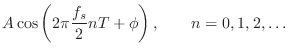
Let's go for broke and plug the general sinusoid into Eq.![]() (1.1),
confident that a table of trigonometry identities will see us through
(after all, this is the simplest filter there is, right?). To set the
input signal to a completely arbitrary sinusoid at amplitude
(1.1),
confident that a table of trigonometry identities will see us through
(after all, this is the simplest filter there is, right?). To set the
input signal to a completely arbitrary sinusoid at amplitude ![]() ,
phase
,
phase ![]() , and frequency
, and frequency ![]() Hz, we let
Hz, we let
![]() . The output is then given by
. The output is then given by
All that remains is to reduce the above expression to a single sinusoid with some frequency-dependent amplitude and phase. We do this first by using standard trigonometric identities [2] in order to avoid introducing complex numbers. Next, a much ``easier'' derivation using complex numbers will be given.
Note that a sum of sinusoids at the same frequency, but possibly different phase and amplitude, can always be expressed as a single sinusoid at that frequency with some resultant phase and amplitude. While we find this result by direct derivation in working out our simple example, the general case is derived in §A.3 for completeness.
We have
| (2.4) |
where
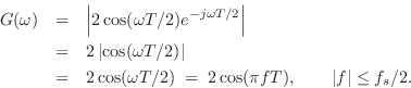
Amplitude Response
We can isolate the filter amplitude response ![]() by squaring
and adding the above two equations:
by squaring
and adding the above two equations:
![\begin{eqnarray*}
a^2(\omega) + b^2(\omega) &=& G^2(\omega)\cos^2[\Theta(\omega)...
...ta(\omega)] + \sin^2[\Theta(\omega)]\right\}\\
&=& G^2(\omega).
\end{eqnarray*}](http://www.dsprelated.com/josimages_new/filters/img165.png)
This can then be simplified as follows:

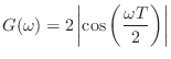
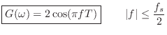
So we have made it to the amplitude response of the simple lowpass
filter
![]() :
:
Phase Response
Now we may isolate the filter phase response
![]() by
taking a ratio of the
by
taking a ratio of the ![]() and
and ![]() in Eq.
in Eq.![]() (1.5):
(1.5):
![\begin{eqnarray*}
\frac{b(\omega)}{a(\omega)}
&=& -\frac{G(\omega) \sin\left[\...
...eft[\Theta(\omega)\right]}\\
&\isdef & - \tan[\Theta(\omega)]
\end{eqnarray*}](http://www.dsprelated.com/josimages_new/filters/img173.png)
Substituting the expansions of ![]() and
and ![]() yields
yields
![\begin{eqnarray*}
\tan[\Theta(\omega)] &=& - \frac{b(\omega)}{a(\omega)} \\
&=&...
...n(\omega T/2)}{\cos(\omega T/2)}
= \tan\left(-\omega T/2\right).
\end{eqnarray*}](http://www.dsprelated.com/josimages_new/filters/img174.png)
Thus, the phase response of the simple lowpass filter
![]() is
is
We have completely solved for the frequency response of the simplest low-pass filter given in Eq.
An Easier Way
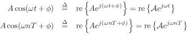
We derived the frequency response above using trig identities in order to minimize the mathematical level involved. However, it turns out it is actually easier, though more advanced, to use complex numbers for this purpose. To do this, we need Euler's identity:
where
Complex Sinusoids
Using Euler's identity to represent sinusoids, we have
when time
Any function of the form
![]() or
or
![]() will henceforth be called a complex
sinusoid.2.3 We will
see that it is easier to manipulate both sine and
cosine simultaneously in this form than it is to deal with
either
sine or cosine separately. One may even take the
point of view that
will henceforth be called a complex
sinusoid.2.3 We will
see that it is easier to manipulate both sine and
cosine simultaneously in this form than it is to deal with
either
sine or cosine separately. One may even take the
point of view that
![]() is simpler and more
fundamental than
is simpler and more
fundamental than
![]() or
or
![]() , as evidenced by
the following identities (which are immediate consequences of Euler's
identity,
Eq.
, as evidenced by
the following identities (which are immediate consequences of Euler's
identity,
Eq.![]() (1.8)):
(1.8)):


Thus, sine and cosine may each be regarded as a combination of two complex sinusoids. Another reason for the success of the complex sinusoid is that we will be concerned only with real linear operations on signals. This means that
Complex Amplitude
Note that the amplitude ![]() and phase
and phase ![]() can be viewed as the
magnitude and angle of a single complex number
can be viewed as the
magnitude and angle of a single complex number
Phasor Notation
The complex amplitude
![]() is also defined as the
phasor associated with any sinusoid having amplitude
is also defined as the
phasor associated with any sinusoid having amplitude ![]() and
phase
and
phase ![]() . The term ``phasor'' is more general than ``complex
amplitude'', however, because it also applies to the corresponding
real sinusoid given by the real part of Equations (1.9-1.10).
In other words, the real sinusoids
. The term ``phasor'' is more general than ``complex
amplitude'', however, because it also applies to the corresponding
real sinusoid given by the real part of Equations (1.9-1.10).
In other words, the real sinusoids
![]() and
and
![]() may be expressed as
may be expressed as
and ![]() is the associated phasor in each case. Thus, we say that
the phasor representation of
is the associated phasor in each case. Thus, we say that
the phasor representation of
![]() is
is
![]() . Phasor analysis is
often used to analyze linear time-invariant systems such as analog
electrical circuits.
. Phasor analysis is
often used to analyze linear time-invariant systems such as analog
electrical circuits.
Plotting Complex Sinusoids as Circular Motion
Figure 1.8 shows Euler's relation graphically as it applies to
sinusoids. A point traveling with uniform velocity around a circle
with radius 1 may be represented by
![]() in
the complex plane, where
in
the complex plane, where ![]() is time and
is time and ![]() is the number of
revolutions per second. The projection of this motion onto the
horizontal (real) axis is
is the number of
revolutions per second. The projection of this motion onto the
horizontal (real) axis is
![]() , and the projection onto
the vertical (imaginary) axis is
, and the projection onto
the vertical (imaginary) axis is
![]() . For
discrete-time circular motion, replace
. For
discrete-time circular motion, replace ![]() by
by ![]() to get
to get
![]() which may be interpreted as a
point which jumps an arc length
which may be interpreted as a
point which jumps an arc length
![]() radians along the circle
each sampling instant.
radians along the circle
each sampling instant.
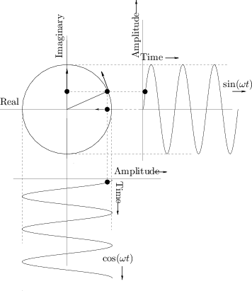 |
For circular motion to ensue, the sinusoidal motions must be at the same frequency, one-quarter cycle out of phase, and perpendicular (orthogonal) to each other. (With phase differences other than one-quarter cycle, the motion is generally elliptical.)
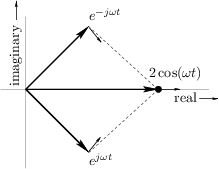
The converse of this is also illuminating. Take the usual circular
motion
![]() which spins counterclockwise along the unit
circle as
which spins counterclockwise along the unit
circle as ![]() increases, and add to it a similar but clockwise
circular motion
increases, and add to it a similar but clockwise
circular motion
![]() . This is shown in
Fig.1.9. Next apply Euler's identity to get
. This is shown in
Fig.1.9. Next apply Euler's identity to get
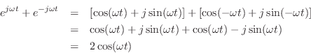
Thus,
This statement is a graphical or geometric interpretation of Eq.
We call
![]() a
positive-frequency sinusoidal component
when
a
positive-frequency sinusoidal component
when
![]() , and
, and
![]() is the
corresponding negative-frequency component. Note that both
sine and cosine signals have equal-amplitude positive- and
negative-frequency components (see also [84,53]). This
happens to be true of every real signal (i.e., non-complex). To
see this, recall that every signal can be represented as a sum of
complex sinusoids at various frequencies (its Fourier
expansion). For the signal to be real, every positive-frequency
complex sinusoid must be summed with a negative-frequency sinusoid of
equal amplitude. In other words, any counterclockwise circular motion
must be matched by an equal and opposite clockwise circular motion in
order that the imaginary parts always cancel to yield a real signal
(see Fig.1.9). Thus, a real signal always has a magnitude
spectrum which is symmetric about 0 Hz. Fourier symmetries such as
this are developed more completely in [84].
is the
corresponding negative-frequency component. Note that both
sine and cosine signals have equal-amplitude positive- and
negative-frequency components (see also [84,53]). This
happens to be true of every real signal (i.e., non-complex). To
see this, recall that every signal can be represented as a sum of
complex sinusoids at various frequencies (its Fourier
expansion). For the signal to be real, every positive-frequency
complex sinusoid must be summed with a negative-frequency sinusoid of
equal amplitude. In other words, any counterclockwise circular motion
must be matched by an equal and opposite clockwise circular motion in
order that the imaginary parts always cancel to yield a real signal
(see Fig.1.9). Thus, a real signal always has a magnitude
spectrum which is symmetric about 0 Hz. Fourier symmetries such as
this are developed more completely in [84].
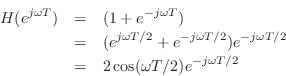
Rederiving the Frequency Response
Let's repeat the mathematical sine-wave analysis of the simplest
low-pass filter, but this time using a complex sinusoid instead of a
real one. Thus, we will test the filter's response at frequency ![]() by setting its input to
by setting its input to
Using the normal rules for manipulating exponents, we find that the
output of the simple low-pass filter in response to the complex
sinusoid at frequency
![]() Hz is given by
Hz is given by
where we have defined
![]() , which we
will show is in fact the frequency response of this filter at
frequency
, which we
will show is in fact the frequency response of this filter at
frequency ![]() . This derivation is clearly easier than the
trigonometry approach. What may be puzzling at first, however, is
that the filter is expressed as a frequency-dependent complex
multiply (when the input signal is a complex sinusoid). What does
this mean? Well, the theory we are blindly trusting at this point
says it must somehow mean a gain scaling and a phase shift. This is
true and easy to see once the complex filter gain is expressed in
polar form,
. This derivation is clearly easier than the
trigonometry approach. What may be puzzling at first, however, is
that the filter is expressed as a frequency-dependent complex
multiply (when the input signal is a complex sinusoid). What does
this mean? Well, the theory we are blindly trusting at this point
says it must somehow mean a gain scaling and a phase shift. This is
true and easy to see once the complex filter gain is expressed in
polar form,
It is now easy to see that
and

It deserves to be emphasized that all a linear time-invariant filter
can do to a sinusoid is scale its amplitude and change
its phase. Since a sinusoid is completely determined by its amplitude
![]() , frequency
, frequency ![]() , and phase
, and phase ![]() , the constraint on the filter is
that the output must also be a sinusoid, and furthermore it must be at
the same frequency as the input sinusoid. More explicitly:
, the constraint on the filter is
that the output must also be a sinusoid, and furthermore it must be at
the same frequency as the input sinusoid. More explicitly:
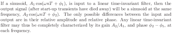
Mathematically, a sinusoid has no beginning and no end, so there really are no start-up transients in the theoretical setting. However, in practice, we must approximate eternal sinusoids with finite-time sinusoids whose starting time was so long ago that the filter output is essentially the same as if the input had been applied forever.
Tying it all together, the general output of a linear time-invariant filter with a complex sinusoidal input may be expressed as
![\begin{eqnarray*}
y(n) &=& (\textit{Complex Filter Gain}) \;\textit{times}\;\, (...
...ith Radius $[G(\omega)A]$\ and Phase $[\phi + \Theta(\omega)]$}.
\end{eqnarray*}](http://www.dsprelated.com/josimages_new/filters/img241.png)
Summary
This chapter has introduced many of the concepts associated with
digital filters, such as signal representations, filter
representations, difference equations, signal flow graphs, software
implementations, sine-wave analysis (real and complex), frequency
response, amplitude response, phase response, and other related
topics. We used a simple filter example to motivate the need for more
advanced methods to analyze digital filters of arbitrary complexity.
We found even in the simple example of Eq.![]() (1.1) that complex
variables are much more compact and convenient for representing
signals and analyzing filters than are trigonometric techniques. We
employ a complex sinusoid
(1.1) that complex
variables are much more compact and convenient for representing
signals and analyzing filters than are trigonometric techniques. We
employ a complex sinusoid
![]() having three
parameters: amplitude, phase, and frequency, and when we put a complex
sinusoid into any linear time-invariant digital filter, the filter
behaves as a simple complex gain
having three
parameters: amplitude, phase, and frequency, and when we put a complex
sinusoid into any linear time-invariant digital filter, the filter
behaves as a simple complex gain
![]() , where the magnitude
, where the magnitude ![]() and
phase
and
phase
![]() are the amplitude response and phase response,
respectively, of the filter.
are the amplitude response and phase response,
respectively, of the filter.
Elementary Filter Theory Problems
See http://ccrma.stanford.edu/~jos/filtersp/Elementary_Filter_Theory_Problems.html.
Next Section:
Matlab Analysis of the Simplest Lowpass Filter
Previous Section:
Preface


