


Cylinder with Conical Cap
Consider a cylindrical acoustic tube adjoined to a converging conical cap, as depicted in Figure C.48a. We may consider the cylinder to be either open or closed on the left side, but everywhere else it is closed. Since such a physical system is obviously passive, an interesting test of acoustic theory is to check whether theory predicts passivity in this case.
![\includegraphics[scale=0.9]{eps/cylconesp}](http://www.dsprelated.com/josimages_new/pasp/img4359.png) |
It is well known that a growing exponential appears at the junction of two conical waveguides when the waves in one conical taper angle reflect from a section with a smaller (or more negative) taper angle [7,300,8,160,9]. The most natural way to model a growing exponential in discrete time is to use an unstable one-pole filter [506]. Since unstable filters do not normally correspond to passive systems, we might at first expect passivity to not be predicted. However, it turns out that all unstable poles are ultimately canceled, and the model is stable after all, as we will see. Unfortunately, as is well known in the field of automatic control, it is not practical to attempt to cancel an unstable pole in a real system, even when it is digital. This is because round-off errors will grow exponentially in the unstable feedback loop and eventually dominate the output.
The need for an unstable filter to model reflection and transmission at a converging conical junction has precluded the use of a straightforward recursive filter model [406]. Using special ``truncated infinite impulse response'' (TIIR) digital filters [540], an unstable recursive filter model can in fact be used in practice [528]. All that is then required is that the infinite-precision system be passive, and this is what we will show in the special case of Fig.C.48.
Scattering Filters at the Cylinder-Cone Junction
As derived in §C.18.4, the wave impedance (for volume velocity)
at frequency ![]() rad/sec in a converging cone is given by
rad/sec in a converging cone is given by
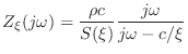 |
(C.152) |
where
(where
The reflectance and transmittance from the right of the junction are the same when there is no wavefront area discontinuity at the junction [300]. Both
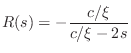
Reflectance of the Conical Cap
Let
![]() denote the time to propagate across the length of
the cone in one direction. As is well known [22], the reflectance
at the tip of an infinite cone is
denote the time to propagate across the length of
the cone in one direction. As is well known [22], the reflectance
at the tip of an infinite cone is ![]() for pressure waves. I.e., it
reflects like an open-ended cylinder. We ignore any absorption losses
propagating in the cone, so that the transfer function from the entrance of
the cone to the tip is
for pressure waves. I.e., it
reflects like an open-ended cylinder. We ignore any absorption losses
propagating in the cone, so that the transfer function from the entrance of
the cone to the tip is
![]() . Similarly, the transfer function from
the conical tip back to the entrance is also
. Similarly, the transfer function from
the conical tip back to the entrance is also
![]() . The complete
reflection transfer function from the entrance to the tip and back is then
. The complete
reflection transfer function from the entrance to the tip and back is then
| (C.155) |
Note that this is the reflectance a distance
We now want to interface the conical cap reflectance
![]() to the
cylinder. Since this entails a change in taper angle, there will be
reflection and transmission filtering at the cylinder-cone junction given
by Eq.
to the
cylinder. Since this entails a change in taper angle, there will be
reflection and transmission filtering at the cylinder-cone junction given
by Eq.![]() (C.154) and Eq.
(C.154) and Eq.![]() (C.155).
(C.155).
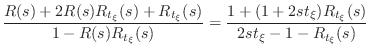
From inside the cylinder, immediately next to the cylinder-cone
junction shown in Fig.C.48, the reflectance of the conical cap is
readily derived from Fig.C.48b and Equations (C.154) and
(C.155) to be
 |
|||
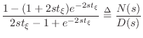 |
(C.156) |
where
| (C.157) |
is the numerator of the conical cap reflectance, and
| (C.158) |
is the denominator. Note that for very large
Stability Proof
A transfer function
![]() is stable if there are no poles in
the right-half
is stable if there are no poles in
the right-half ![]() plane. That is, for each zero
plane. That is, for each zero ![]() of
of ![]() , we must
have
re
, we must
have
re![]() . If this can be shown, along with
. If this can be shown, along with
![]() , then the reflectance
, then the reflectance ![]() is shown to be
passive. We must also study the system zeros (roots of
is shown to be
passive. We must also study the system zeros (roots of ![]() ) in order to
determine if there are any pole-zero cancellations (common factors in
) in order to
determine if there are any pole-zero cancellations (common factors in
![]() and
and ![]() ).
).
Since
re![]() if and only if
re
if and only if
re![]() , for
, for
![]() , we may set
, we may set
![]() without loss of generality. Thus, we need only
study the roots of
without loss of generality. Thus, we need only
study the roots of
If this system is stable, we have stability also for all
![]() .
Since
.
Since ![]() is not a rational function of
is not a rational function of ![]() , the reflectance
, the reflectance ![]() may have infinitely many poles and zeros.
may have infinitely many poles and zeros.
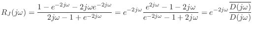
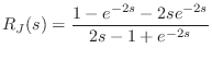
Let's first consider the roots of the denominator
| (C.159) |
At any solution

To obtain separate equations for the real and imaginary parts, set
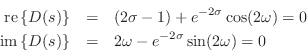
Both of these equations must hold at any pole of the reflectance. For
stability, we further require
![]() . Defining
. Defining
![]() and
and
![]() , we obtain the somewhat simpler conditions
, we obtain the somewhat simpler conditions
For any poles of ![]() on the
on the ![]() axis, we have
axis, we have ![]() , and
Eq.
, and
Eq.![]() (C.163) reduces to
(C.163) reduces to
It is well known that the ``sinc function''
We have so far proved that any poles on the ![]() axis must be at
axis must be at
![]() .
.
The same argument can be extended to the entire right-half
plane as follows. Going back to the more general case of
Eq.![]() (C.163), we have
(C.163), we have
 |
(C.164) |
Since
In the left-half plane, there are many potential poles.
Equation (C.162) has infinitely many solutions for each ![]() since the elementary inequality
since the elementary inequality
![]() implies
implies
![]() . Also, Eq.
. Also, Eq.![]() (C.163) has an increasing
number of solutions as
(C.163) has an increasing
number of solutions as ![]() grows more and more negative; in the limit of
grows more and more negative; in the limit of
![]() , the number of solutions is infinite and given by the roots
of
, the number of solutions is infinite and given by the roots
of ![]() (
(
![]() for any integer
for any integer ![]() ).
However, note that at
).
However, note that at
![]() , the solutions of Eq.
, the solutions of Eq.![]() (C.162) converge to the roots of
(C.162) converge to the roots of
![]() (
(
![]() for any integer
for any integer ![]() ).
The only issue is that the solutions of Eq.
).
The only issue is that the solutions of Eq.![]() (C.162) and Eq.
(C.162) and Eq.![]() (C.163)
must occur together.
(C.163)
must occur together.
![\includegraphics[width=3.5in]{eps/cylconelhp}](http://www.dsprelated.com/josimages_new/pasp/img4420.png) |
Figure C.49 plots the locus of real-part zeros (solutions to
Eq.![]() (C.162)) and imaginary-part zeros (Eq.
(C.162)) and imaginary-part zeros (Eq.![]() (C.163)) in a portion
the left-half plane. The roots at
(C.163)) in a portion
the left-half plane. The roots at ![]() can be seen at the
middle-right. Also, the asymptotic interlacing of these loci can be
seen along the left edge of the plot. It is clear that the two loci
must intersect at infinitely many points in the left-half plane near
the intersections indicated in the graph. As
can be seen at the
middle-right. Also, the asymptotic interlacing of these loci can be
seen along the left edge of the plot. It is clear that the two loci
must intersect at infinitely many points in the left-half plane near
the intersections indicated in the graph. As
![]() becomes
large, the intersections evidently converge to the peaks of the
imaginary-part root locus (a log-sinc function rotated
90 degrees). At all frequencies
becomes
large, the intersections evidently converge to the peaks of the
imaginary-part root locus (a log-sinc function rotated
90 degrees). At all frequencies ![]() , the roots occur near
the log-sinc peaks, getting closer to the peaks as
, the roots occur near
the log-sinc peaks, getting closer to the peaks as
![]() increases. The log-sinc peaks thus provide a reasonable estimate
number and distribution in the left-half
increases. The log-sinc peaks thus provide a reasonable estimate
number and distribution in the left-half ![]() -plane. An outline of an
analytic proof is as follows:
-plane. An outline of an
analytic proof is as follows:
- Rotate the loci in Fig.C.49 counterclockwise by 90 degrees.
- Prove that the two root loci are continuous, single-valued functions of
 (as the figure suggests).
- Prove that for
 , there are infinitely many extrema
of the log-sinc function (imaginary-part root-locus) which have
negative curvature and which lie below
, there are infinitely many extrema
of the log-sinc function (imaginary-part root-locus) which have
negative curvature and which lie below  (as the figure
suggests). The
(as the figure
suggests). The  and
and  lines are shown in the
figure as dotted lines.
lines are shown in the
figure as dotted lines.
- Prove that the other root locus (for the real part) has
infinitely many similar extrema which occur for
 (again as
the figure suggests).
(again as
the figure suggests).
- Prove that the two root-loci interlace at
 (already done above).
- Then topologically, the continuous functions must cross at
infinitely many points in order to achieve interlacing at
.
The peaks of the log-sinc function not only indicate approximately where the left-half-plane roots occur
Reflectance Magnitude
We have shown that the conical cap reflectance has no poles in the
strict right-half plane. For passivity, we also need to show that its
magnitude is bounded by unity for all ![]() on the
on the ![]() axis.
axis.
We have
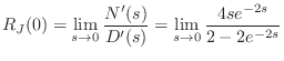
Poles at 
We know from the above that the denominator of the cone reflectance
has at least one root at ![]() . In this subsection we investigate
this ``dc behavior'' of the cone more thoroughly.
. In this subsection we investigate
this ``dc behavior'' of the cone more thoroughly.
A hasty analysis based on the reflection and transmission filters in
Equations (C.154) and (C.155) might conclude that the reflectance
of the conical cap converges to ![]() at dc, since
at dc, since ![]() and
and ![]() .
However, this would be incorrect. Instead, it is necessary to take the
limit as
.
However, this would be incorrect. Instead, it is necessary to take the
limit as
![]() of the complete conical cap reflectance
of the complete conical cap reflectance ![]() :
:
 |
(C.165) |
We already discovered a root at
 |
(C.166) |
and once again the limit is an indeterminate
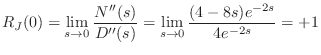 |
(C.167) |
Thus, two poles and zeros cancel at dc, and the dc reflectance is
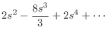
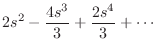
Another method of showing this result is to form a Taylor series expansion
of the numerator and denominator:
 |
(C.168) | ||
 |
(C.169) |
Both series begin with the term
 |
(C.170) |
which approaches
An alternative analysis of this issue is given by Benade in [37].
Next Section:
Consistency
Previous Section:
Generalized Scattering Coefficients


