


Optimal Peak-Finding in the Spectrum
Based on the preceding sections, an ``obvious'' method for deducing sinusoidal parameters from data is to find the amplitude, phase, and frequency of each peak in a zero-padded FFT of the data. We have considered so far the following issues:
- Make sure the data length (or window length) is long enough so that all sinusoids in the data are resolved.
- Use enough zero padding so that the spectrum is heavily oversampled, making the peaks easier to interpolate.
- Use quadratic interpolation of the three samples surrounding a dB-magnitude peak in the heavily oversampled spectrum.
- Evaluate the fitted parabola at its extremum to obtain the interpolated amplitude and frequency estimates for each sinusoidal component.
- Similarly compute a phase estimate at each peak frequency using quadratic or even linear interpolation on the unwrapped phase samples about the peak.
The question naturally arises as to how good is the QIFFT method for spectral peak estimation? Is it optimal in any sense? Are there better methods? Are there faster methods that are almost as good? These are questions that generally fall under the topic of sinusoidal parameter estimation.
We will show that the QIFFT method is a fast, ``approximate maximum-likelihood method.'' When properly configured, it is in fact extremely close to the true maximum-likelihood estimator for a single sinusoid in white noise. It is also close to the maximum likelihood estimator for multiple sinusoids that are well separated in frequency (i.e., side-lobe overlap can be neglected). Finally, the QIFFT method can be considered optimal perceptually in the sense that any errors induced by the suboptimality of the QIFFT method are inaudible when the zero-padding factor is a factor of 5 or more. While a zero-padding factor of 5 is sufficient for all window types, including the rectangular window, less zero-padding is needed with windows having flatter main-lobe peaks, as summarized in Table 5.3.
Minimum Zero-Padding for High-Frequency Peaks
|
Table 5.3 gives zero-padding factors sufficient for keeping
the bias below
![]() Hz, where
Hz, where ![]() denotes the sampling
rate in Hz, and
denotes the sampling
rate in Hz, and ![]() is the window length in samples. For fundamental
frequency estimation,
is the window length in samples. For fundamental
frequency estimation, ![]() can be interpreted as the
relative frequency error ``
can be interpreted as the
relative frequency error ``
![]() '' when the window
length is one period. In this case,
'' when the window
length is one period. In this case, ![]() is the fundamental
frequency in Hz. More generally,
is the fundamental
frequency in Hz. More generally, ![]() is the bandwidth of each
side-lobe in the DTFT of a length
is the bandwidth of each
side-lobe in the DTFT of a length ![]() rectangular, generalized
Hamming, or Blackman window (any member of the Blackman-Harris window
family, as elaborated in Chapter 3).
rectangular, generalized
Hamming, or Blackman window (any member of the Blackman-Harris window
family, as elaborated in Chapter 3).
Note from Table 5.3 that the Blackman window requires no
zero-padding at all when only ![]() % accuracy is required in
peak-frequency measurement. It should also be understood that a
frequency error of
% accuracy is required in
peak-frequency measurement. It should also be understood that a
frequency error of ![]() % is inaudible in most audio
applications.6.10
% is inaudible in most audio
applications.6.10
Minimum Zero-Padding for Low-Frequency Peaks
Sharper bounds on the zero-padding factor needed for low-frequency
peaks (below roughly 1 kHz) may be obtained based on the measured
Just-Noticeable-Difference (JND) in frequency and/or amplitude
[276]. In particular, a ![]() % relative-error
spec is good above 1 kHz (being conservative by approximately a factor
of 2), but overly conservative at lower frequencies where the JND
flattens out. Below 1 kHz, a fixed 1 Hz spec satisfies perceptual
requirements and gives smaller minimum zero-padding factors than the
% relative-error
spec is good above 1 kHz (being conservative by approximately a factor
of 2), but overly conservative at lower frequencies where the JND
flattens out. Below 1 kHz, a fixed 1 Hz spec satisfies perceptual
requirements and gives smaller minimum zero-padding factors than the
![]() % relative-error spec.
% relative-error spec.
The following data, extracted from [276, Table I, p. 89] gives frequency JNDs at a presentation level of 60 dB SPL (the most sensitive case measured):
  f =    [    62,    125,    250,    500,   1000,   2000,   4000];
  dfof = [0.0346, 0.0269, 0.0098, 0.0035, 0.0034, 0.0018, 0.0020];
Thus, the frequency JND at 4 kHz was measured to be two tenths of a percent. (These measurements were made by averaging experimental results for five men between the ages of 20 and 30.) Converting relative frequency to absolute frequency in Hz yields (in matlab syntax):
df = dfof .* f; % = [2.15, 3.36, 2.45, 1.75, 3.40, 3.60, 8.00];For purposes of computing the minimum zero-padding factor required, we see that the absolute tuning error due to bias can be limited to 1 Hz, based on measurements at 500 Hz (at 60 dB). Doing this for frequencies below 1 kHz yields the results shown in Table 5.4. Note that the Blackman window needs no zero padding below 125 Hz, and the Hamming/Hann window requires no zero padding below 62.5 Hz.
|
Matlab for Computing Minimum Zero-Padding Factors
The minimum zero-padding factors in the previous two subsections were computed using the matlab function zpfmin listed in §F.2.4. For example, both tables above are included in the output of the following matlab program:
  windows={'rect','hann','hamming','blackman'};
  freqs=[1000,500,250,125,62.5];
  for i=1:length(windows)
    w = sprintf("%s",windows(i))
    for j=1:length(freqs)
      f = freqs(j);
      zpfmin(w,1/f,0.01*f)  % 1 percent spec (large for audio)
      zpfmin(w,1/f,0.001*f) % 0.1 percent spec (good > 1 kHz)
      zpfmin(w,1/f,1)       % 1 Hz spec (good below 1 kHz)
    end
  end
In addition to ``perceptually exact'' detection of spectral peaks, there are times when we need to find spectral parameters as accurately as possible, irrespective of perception. For example, one can estimate the stiffness of a piano string by measuring the stretched overtone-frequencies in the spectrum of that string's vibration. Additionally, we may have measurement noise, in which case we want our measurements to be minimally influenced by this noise. The following sections discuss optimal estimation of spectral-peak parameters due to sinusoids in the presence of noise.
Least Squares Sinusoidal Parameter Estimation
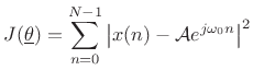
There are many ways to define ``optimal'' in signal modeling. Perhaps the most elementary case is least squares estimation. Every estimator tries to measure one or more parameters of some underlying signal model. In the case of sinusoidal parameter estimation, the simplest model consists of a single complex sinusoidal component in additive white noise:
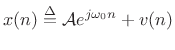
where
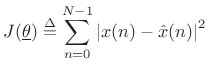
with respect to the parameter vector
![$\displaystyle \underline{\theta}\isdef \left[\begin{array}{c} A \\ [2pt] \phi \\ [2pt] \omega_0 \end{array}\right],$](http://www.dsprelated.com/josimages_new/sasp2/img1033.png) |
(6.34) |
where
 |
(6.35) |
Note that the error signal
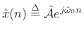
Sinusoidal Amplitude Estimation
If the sinusoidal frequency ![]() and phase
and phase ![]() happen to be
known, we obtain a simple linear least squares problem for the
amplitude
happen to be
known, we obtain a simple linear least squares problem for the
amplitude ![]() . That is, the error signal
. That is, the error signal
| (6.36) |
becomes linear in the unknown parameter
becomes a simple quadratic (parabola) over the real line.6.11 Quadratic forms in any number of dimensions are easy to minimize. For example, the ``bottom of the bowl'' can be reached in one step of Newton's method. From another point of view, the optimal parameter
Yet a third way to minimize (5.37) is the method taught in
elementary calculus: differentiate
![]() with respect to
with respect to ![]() , equate
it to zero, and solve for
, equate
it to zero, and solve for ![]() . In preparation for this, it is helpful to
write (5.37) as
. In preparation for this, it is helpful to
write (5.37) as
![\begin{eqnarray*}
J({\hat A}) &\isdef & \sum_{n=0}^{N-1}
\left[x(n)-{\hat A}e^{j(\omega_0 n+\phi)}\right]
\left[\overline{x(n)}-\overline{{\hat A}} e^{-j(\omega_0 n+\phi)}\right]\\
&=&
\sum_{n=0}^{N-1}
\left[
\left\vert x(n)\right\vert^2
-
x(n)\overline{{\hat A}} e^{-j(\omega_0 n+\phi)}
-
\overline{x(n)}{\hat A}e^{j(\omega_0 n+\phi)}
+
{\hat A}^2
\right]
\\
&=& \left\Vert\,x\,\right\Vert _2^2 - 2\mbox{re}\left\{\sum_{n=0}^{N-1} x(n)\overline{{\hat A}}
e^{-j(\omega_0 n+\phi)}\right\}
+ N {\hat A}^2.
\end{eqnarray*}](http://www.dsprelated.com/josimages_new/sasp2/img1045.png)
Differentiating with respect to ![]() and equating to zero yields
and equating to zero yields
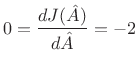 re re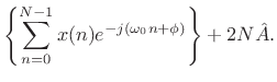 |
(6.38) |
Solving this for
 re
re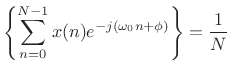 re
reThat is, the optimal least-squares amplitude estimate may be found by the following steps:
- Multiply the data
 by
by
 to zero the known phase
  .
.
- Take the DFT of the
 samples of
  , suitably zero padded to approximate the DTFT, and evaluate it at the known frequency
  .
.
- Discard any imaginary part since it can only contain noise, by (5.39).
- Divide by
to obtain a properly normalized coefficient of projection
[264] onto the sinusoid
(6.40)
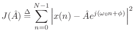
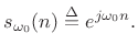
Sinusoidal Amplitude and Phase Estimation
The form of the optimal estimator (5.39) immediately suggests the following generalization for the case of unknown amplitude and phase:
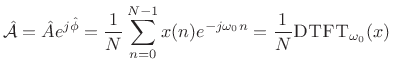
That is,
The orthogonality principle for linear least squares estimation states
that the projection error must be orthogonal to the model.
That is, if ![]() is our optimal signal model (viewed now as an
is our optimal signal model (viewed now as an
![]() -vector in
-vector in ![]() ), then we must have [264]
), then we must have [264]

Thus, the complex coefficient of projection of ![]() onto
onto
![]() is given by
is given by
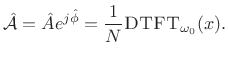 |
(6.42) |
The optimality of
 |
Sinusoidal Frequency Estimation
The form of the least-squares estimator (5.41) in the known-frequency case immediately suggests the following frequency estimator for the unknown-frequency case:
That is, the sinusoidal frequency estimate is defined as that frequency which maximizes the DTFT magnitude. Given this frequency, the least-squares sinusoidal amplitude and phase estimates are given by (5.41) evaluated at that frequency.
It can be shown [121] that (5.43) is in fact the optimal least-squares estimator for a single sinusoid in white noise. It is also the maximum likelihood estimator for a single sinusoid in Gaussian white noise, as discussed in the next section.
In summary,
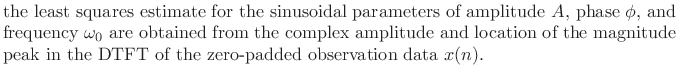
In practice, of course, the DTFT is implemented as an interpolated FFT, as described in the previous sections (e.g., QIFFT method).
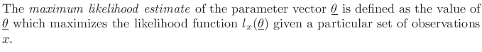
Maximum Likelihood Sinusoid Estimation
The maximum likelihood estimator (MLE) is widely used in practical signal modeling [121]. A full treatment of maximum likelihood estimators (and statistical estimators in general) lies beyond the scope of this book. However, we will show that the MLE is equivalent to the least squares estimator for a wide class of problems, including well resolved sinusoids in white noise.
Consider again the signal model of (5.32) consisting of a complex sinusoid in additive white (complex) noise:
Again,
 |
(6.46) |
We express the zero-mean Gaussian assumption by writing
| (6.47) |
The parameter
It turns out that when Gaussian random variables ![]() are
uncorrelated (i.e., when
are
uncorrelated (i.e., when ![]() is white noise), they are also
independent. This means that the probability of observing
particular values of
is white noise), they are also
independent. This means that the probability of observing
particular values of ![]() and
and ![]() is given by the product of
their respective probabilities [121]. We will now use this
fact to compute an explicit probability for observing any data
sequence
is given by the product of
their respective probabilities [121]. We will now use this
fact to compute an explicit probability for observing any data
sequence ![]() in (5.44).
in (5.44).
Since the sinusoidal part of our signal model,
![]() , is deterministic; i.e., it does not including any random
components; it may be treated as the time-varying mean of a
Gaussian random process
, is deterministic; i.e., it does not including any random
components; it may be treated as the time-varying mean of a
Gaussian random process ![]() . That is, our signal model
(5.44) can be rewritten as
. That is, our signal model
(5.44) can be rewritten as
| (6.48) |
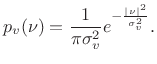
and the probability density function for the whole set of observations
![$\displaystyle p(x) = p[x(0)] p[x(1)]\cdots p[x(N-1)] = \left(\frac{1}{\pi \sigma_v^2}\right)^N e^{-\frac{1}{\sigma_v^2}\sum_{n=0}^{N-1} \left\vert x(n) - {\cal A}e^{j\omega_0 n}\right\vert^2}$](http://www.dsprelated.com/josimages_new/sasp2/img1079.png) |
(6.49) |
Thus, given the noise variance
Likelihood Function
The likelihood function
![]() is defined as the
probability density function of
is defined as the
probability density function of ![]() given
given
![]() , evaluated at a particular
, evaluated at a particular ![]() , with
, with
![]() regarded as a variable.
regarded as a variable.
In other words, the likelihood function
![]() is just the PDF
of
is just the PDF
of ![]() with a particular value of
with a particular value of ![]() plugged in, and any parameters
in the PDF (mean and variance in this case) are treated as variables.
plugged in, and any parameters
in the PDF (mean and variance in this case) are treated as variables.
For the sinusoidal parameter estimation problem, given a set of
observed data samples ![]() , for
, for
![]() , the likelihood
function is
, the likelihood
function is
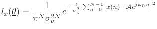 |
(6.50) |
and the log likelihood function is
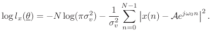 |
(6.51) |
We see that the maximum likelihood estimate for the parameters of a sinusoid in Gaussian white noise is the same as the least squares estimate. That is, given
 |
(6.52) |
as we saw before in (5.33).
Multiple Sinusoids in Additive Gaussian White Noise
The preceding analysis can be extended to the case of multiple sinusoids in white noise [120]. When the sinusoids are well resolved, i.e., when window-transform side lobes are negligible at the spacings present in the signal, the optimal estimator reduces to finding multiple interpolated peaks in the spectrum.
One exact special case is when the sinusoid frequencies ![]() coincide with the ``DFT frequencies''
coincide with the ``DFT frequencies''
![]() , for
, for
![]() . In this special case, each sinusoidal peak sits
atop a zero crossing in the window transform associated with every
other peak.
. In this special case, each sinusoidal peak sits
atop a zero crossing in the window transform associated with every
other peak.
To enhance the ``isolation'' among multiple sinusoidal peaks, it is natural to use a window function which minimizes side lobes. However, this is not optimal for short data records since valuable data are ``down-weighted'' in the analysis. Fundamentally, there is a trade-off between peak estimation error due to overlapping side lobes and that due to widening the main lobe. In a practical sinusoidal modeling system, not all sinusoidal peaks are recovered from the data--only the ``loudest'' peaks are measured. Therefore, in such systems, it is reasonable to assure (by choice of window) that the side-lobe level is well below the ``cut-off level'' in dB for the sinusoidal peaks. This prevents side lobes from being comparable in magnitude to sinusoidal peaks, while keeping the main lobes narrow as possible.
When multiple sinusoids are close together such that the associated main lobes overlap, the maximum likelihood estimator calls for a nonlinear optimization. Conceptually, one must search over the possible superpositions of the window transform at various relative amplitudes, phases, and spacings, in order to best ``explain'' the observed data.
Since the number of sinusoids present is usually not known, the number can be estimated by means of hypothesis testing in a Bayesian framework [21]. The ``null hypothesis'' can be ``no sinusoids,'' meaning ``just white noise.''
Non-White Noise
The noise process ![]() in (5.44) does not have to be white
[120]. In the non-white case, the spectral shape of the noise
needs to be estimated and ``divided out'' of the spectrum. That is, a
``pre-whitening filter'' needs to be constructed and applied to the
data, so that the noise is made white. Then the previous case can be
applied.
in (5.44) does not have to be white
[120]. In the non-white case, the spectral shape of the noise
needs to be estimated and ``divided out'' of the spectrum. That is, a
``pre-whitening filter'' needs to be constructed and applied to the
data, so that the noise is made white. Then the previous case can be
applied.
Generality of Maximum Likelihood Least Squares
Note that the maximum likelihood estimate coincides with the least squares estimate whenever the signal model is of the form
| (6.53) |
where
Next Section:
Introduction to Noise
Previous Section:
Sinusoidal Peak Interpolation


