Phase Vocoder Sinusoidal Modeling

Free Books Spectral Audio Signal Processing

As mentioned in §G.7, the phase vocoder had become a standard analysis tool for additive synthesis (§G.8) by the late 1970s [186,187]. This section summarizes that usage.

In analysis for additive synthesis, we convert a time-domain signal into a collection of amplitude envelopes and frequency envelopes $\omega_k+\Delta\omega_k(t)$ (or phase modulation envelopes $\phi_k(t)=\int_t\Delta\omega_k(t)\,dt$ ), as graphed in Fig.G.12. It is usually desired that these envelopes be slowly varying relative to the original signal. This leads to the assumption that we have at most one sinusoid in each filter-bank channel. (By ``sinusoid'' we mean, of course, ``quasi sinusoid,'' since its amplitude and phase may be slowly time-varying.) The channel-filter frequency response is given by the FFT of the analysis window used (Chapter 9).

The signal in the $k^{th}$ subband (filter-bank channel) can be written

$\displaystyle x_k(t)\eqsp a_k(t)\cos[ \omega_kt + \phi_k(t) ]. \protect$

(G.3)

In this expression, is an amplitude modulation term, $\omega_k$ is a fixed channel center frequency, and $\phi_k(t)$ is a phase modulation (or, equivalently, the time-integral of a frequency modulation). Using these parameters, we can resynthesize the signal using the classic oscillator summation, as shown in Fig.10.7 (ignoring the filtered noise in that figure).^G.9

Typically, the instantaneous phase modulation $\phi_k(t)$ is differentiated to obtain instantaneous frequency deviation:

$\displaystyle \Delta \omega_k(t) \isdefs \frac{d}{dt} \phi_k(t)$

(G.4)

The analysis and synthesis signal models are summarized in Fig.G.9.

**Figure G.9:** Illustration of channel vocoder parameters in analysis (left) and synthesis (right).
$\includegraphics[width=\twidth]{eps/pvchan}$

Computing Vocoder Parameters

To compute the amplitude at the output of the th subband, we can apply an envelope follower. Classically, such as in the original vocoder, this can be done by full-wave rectification and subsequent low pass filtering, as shown in Fig.G.10. This produces an approximation of the average power in each subband.

$\begin{psfrags} % latex2html id marker 42527\psfrag{x} []{ \LARGE$ x_k(t)$\ }\psfrag{xkt} []{ \LARGE$ \tilde{x}_k(t)$\ }\psfrag{xk} []{ \LARGE$ x_k(t)$\ }\psfrag{output} []{ \LARGE$ y_k=h*\tilde{x}_k $\ }\begin{figure}[htbp] \includegraphics[width=\textwidth ]{eps/envelope} \caption{Classic method for amplitude envelope extraction in continuous-time analog circuits.} \end{figure} \end{psfrags}$

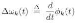
In digital signal processing, we can do much better than the classical amplitude-envelope follower: We can measure instead the instantaneous amplitude of the (assumed quasi sinusoidal) signal in each filter band using so-called analytic signal processing (introduced in §4.6). For this, we generalize (G.3) to the real-part of the corresponding analytic signal:

$\displaystyle x_k(t)\eqsp a_k(t)\cos[ \omega_kt + \phi_k(t) ] \eqsp$ $\displaystyle \mbox{re\ensuremath{\left\{a_k(t)e^{j\phi_k(t)} e^{j\omega_k t}\right\}}}$ $\displaystyle \isdefs$ $\displaystyle \mbox{re\ensuremath{\left\{x^a_k(t)\right\}}}$ $\displaystyle \protect$

(G.5)

In general, when both amplitude and phase are needed, we must compute two real signals for each vocoder channel:

$\displaystyle a_k(t)$	$\displaystyle =$	$\displaystyle \vert x_k^a(t) \vert$ (instantaneous amplitude)
$\displaystyle \phi_k(t)$	$\displaystyle =$	$\displaystyle \angle x_k^a(t) - \omega_kt$ (instantaneous phase)
	$\displaystyle =$	$\displaystyle \tan^{-1} \left[ \frac{\mbox{im\ensuremath{\left\{x_k^a(t)\right\}}}} {\mbox{re\ensuremath{\left\{x_k^a(t)\right\}}}} \right] - \omega_kt \protect$	(G.6)

We call the instantaneous amplitude at time for both and . The function $a_k(\cdot)$ as a whole is called the amplitude envelope of the th channel output. The instantaneous phase at time is $\phi_k(t)$ , and its time-derivative is instantaneous frequency.

In order to determine these signals, we need to compute the analytic signal from its real part . Ideally, the imaginary part of the analytic signal is obtained from its real part using the Hilbert transform (§4.6), as shown in Fig.G.11.

$\begin{psfrags} % latex2html id marker 42563\psfrag{x} []{ \LARGE$ x_k(t)$\ }\psfrag{Rex} []{ \LARGE$ \mbox{re\ensuremath{\left\{x_k^a(t)\right\}}}$\ }\psfrag{Imx} []{ \LARGE$ \mbox{im\ensuremath{\left\{x_k^a(t)\right\}}}$\ }\begin{figure}[htbp] \includegraphics[width=0.8\twidth]{eps/hilbert} \caption{Creating an analytic signal from its real part using the Hilbert transform (\textit{cf.}{} \sref {hilbert}).} \end{figure} \end{psfrags}$

Using the Hilbert-transform filter, we obtain the analytic signal in ``rectangular'' (Cartesian) form:

$\displaystyle x_k^a(t) =$ $\displaystyle \mbox{re\ensuremath{\left\{x_k^a(t)\right\}}}$ $\displaystyle + j\,$ $\displaystyle \mbox{im\ensuremath{\left\{x_k^a(t)\right\}}}$

(G.7)

To obtain the instantaneous amplitude and phase, we simply convert each complex value of to polar form

$\displaystyle x_k^a(t) \eqsp a_k(t)\,e^{j[ \omega_kt +\phi_k(t)] }$

(G.8)

as given by (G.6).

Frequency Envelopes

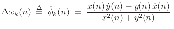
It is convenient in practice to work with instantaneous frequency deviation instead of phase:

$\displaystyle \Delta \omega_k(t) \isdefs \frac{d}{dt} \phi_k(t)$

(G.9)

Since the th channel of an -channel uniform filter-bank has nominal bandwidth given by , the frequency deviation usually does not exceed $\pm f_s/(2N)$ .

Note that is a narrow-band signal centered about the channel frequency $\omega_k$ . As detailed in Chapter 9, it is typical to heterodyne the channel signals to ``base band'' by shifting the input spectrum by $-\omega_k$ so that the channel bandwidth is centered about frequency zero (dc). This may be expressed by modulating the analytic signal by $\exp(-j\omega_k t)$ to get

$\displaystyle x_k^b(t) \isdefs e^{-j\omega_k t}\, x_k^a(t) = a_k(t)\, e^{j\phi_k(t)}$

(G.10)

The `b' superscript here stands for ``baseband,'' i.e., the channel-filter frequency-response is centered about dc. Working at baseband, we may compute the frequency deviation as simply the time-derivative of the instantaneous phase of the analytic signal:

$\displaystyle \Delta\omega_k(t) \isdefs \frac{d}{dt} \angle x_k^b(t) \isdefs \dot{\phi}_k(t)$

(G.11)

where

$\displaystyle \dot{\phi}_k(t) \isdefs \frac{d}{dt} \phi_k(t)$

(G.12)

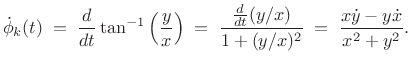denotes the time derivative of $\phi_k(t)$ . For notational simplicity, let $x(t) \isdeftext \mbox{re\ensuremath{\left\{x_k^b(t)\right\}}}$ and $y(t)\isdeftext \mbox{im\ensuremath{\left\{ x_k^b(t)\right\}}}$ . Then we have

$\displaystyle \dot{\phi}_k(t) \eqsp \frac{d}{dt}\tan^{-1}\left(\frac{y}{x}\right) \eqsp \frac{ \frac{d}{dt}{(y/x)}}{ 1+(y/x)^2} \eqsp \frac{x\dot{y}-y\dot{x}}{x^2+y^2} .$

(G.13)

For discrete time, we replace by to obtain [186]

$\displaystyle \Delta\omega_k(n) \isdefs \dot{\phi}_k(n) \eqsp \frac{x(n)\,\dot{y}(n)-y(n)\,\dot{x}(n)}{x^2(n)+y^2(n)}. \protect$

(G.14)

Initially, the sliding FFT was used (hop size in the notation of Chapters 8 and 9). Larger hop sizes can result in phase ambiguities, i.e., it can be ambiguous exactly how many cycles of a quasi-sinusoidal component occurred during the hop within a given channel, especially for high-frequency channels. In many applications, this is not a serious problem, as it is only necessary to recreate a psychoacoustically equivalent peak trajectory in the short-time spectrum. For related discussion, see [299].

Using (G.6) and (G.14) to compute the instantaneous amplitude and frequency for each subband, we obtain data such as shown qualitatively in Fig.G.12. A matlab algorithm for phase unwrapping is given in §F.4.1.

$\begin{psfrags} % latex2html id marker 42622\psfrag{ak} []{ \LARGE$ a_k(t)$\ }\psfrag{wkt} []{ \LARGE$ \Delta\omega_k(t)=\dot{\phi_k}(t) $\ }\psfrag{wk} []{ \LARGE$ 0 $\ }\psfrag{t} []{ \LARGE$ t$\ }\begin{figure}[htbp] \includegraphics[width=3.5in]{eps/traj} \caption{Example amplitude envelope (top) and frequency envelope (bottom).} \end{figure} \end{psfrags}$

Envelope Compression

Once we have our data in the form of amplitude and frequency envelopes for each filter-bank channel, we can compress them by a large factor. If there are channels, we nominally expect to be able to downsample by a factor of , as discussed initially in Chapter 9 and more extensively in Chapter 11.

In early computer music [97,186], amplitude and frequency envelopes were ``downsampled'' by means of piecewise linear approximation. That is, a set of breakpoints were defined in time between which linear segments were used. These breakpoints correspond to ``knot points'' in the context of polynomial spline interpolation [286]. Piecewise linear approximation yielded large compression ratios for relatively steady tonal signals.^G.10For example, compression ratios of 100:1 were not uncommon for isolated ``toots'' on tonal orchestral instruments [97].

A more straightforward method is to simply downsample each envelope by some factor. Since each subband is bandlimited to the channel bandwidth, we expect a downsampling factor on the order of the number of channels in the filter bank. Using a hop size in the STFT results in downsampling by the factor (as discussed in §9.8). If channels are downsampled by , then the total number of samples coming out of the filter bank equals the number of samples going into the filter bank. This may be called critical downsampling, which is invariably used in filter banks for audio compression, as discussed further in Chapter 11. A benefit of converting a signal to critically sampled filter-bank form is that bits can be allocated based on the amount of energy in each subband relative to the psychoacoustic masking threshold in that band. Bit-allocation is typically different for tonal and noise signals in a band [113,25,16].

Vocoder-Based Additive-Synthesis Limitations

Using the phase-vocoder to compute amplitude and frequency envelopes for additive synthesis works best for quasi-periodic signals. For inharmonic signals, the vocoder analysis method can be unwieldy: The restriction of one sinusoid per subband leads to many ``empty'' bands (since radix-2 FFT filter banks are always uniformly spaced). As a result, we have to compute many more filter bands than are actually needed, and the empty bands need to be ``pruned'' in some way (e.g., based on an energy detector within each band). The unwieldiness of a uniform filter bank for tracking inharmonic partial overtones through time led to the development of sinusoidal modeling based on the STFT, as described in §G.11.2 below.

Another limitation of the phase-vocoder analysis was that it did not capture the attack transient very well in the amplitude and frequency envelopes computed. This is because an attack transient typically only partially filled an STFT analysis window. Moreover, filter-bank amplitude and frequency envelopes provide an inefficient model for signals that are noise-like, such as a flute with a breathy attack. These limitations are addressed by sinusoidal modeling, sines+noise modeling, and sines+noise+transients modeling, as discussed starting in §10.4 below (as well as in §10.4).

The phase vocoder was not typically implemented as an identity system due mainly to the large data reduction of the envelopes (piecewise linear approximation). However, it could be used as an identity system by keeping the envelopes at the full signal sampling rate and retaining the initial phase information for each channel. Instantaneous phase is then reconstructed as the initial phase plus the time-integral of the instantaneous frequency (given by the frequency envelope).