


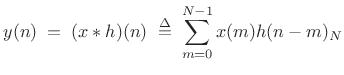
Overlap-Add (OLA) STFT Processing
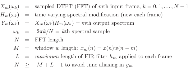
This chapter discusses use of the Short-Time Fourier Transform (STFT) to implement linear filtering in the frequency domain. Due to the speed of FFT convolution, the STFT provides the most efficient single-CPU implementation engine for most FIR filters encountered in audio signal processing.
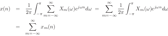
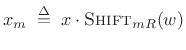
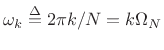
Recall from §7.1 the STFT:
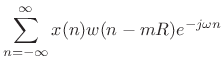
where
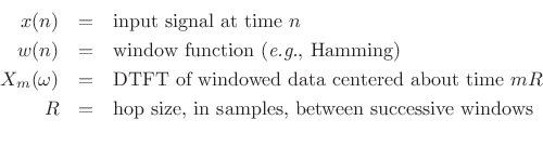
We noted that if the window ![]() has the
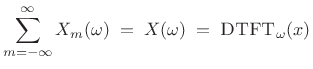
constant overlap-add property
at hop-size
has the
constant overlap-add property
at hop-size ![]() ,
,
 |
(9.2) |
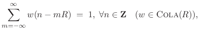
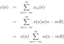
then the sum of the successive DTFTs over time equals the DTFT of the whole signal
 |
(9.3) |
Consequently, the inverse-STFT is simply the inverse-DTFT of this sum:
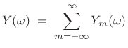
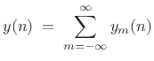
We may now introduce spectral modifications by multiplying each
spectral frame
![]() by some filter frequency response
by some filter frequency response
![]() to get
to get
| (9.4) |
Note that
 |
(9.5) |
so that
 |
(9.6) |
where
| (9.7) |
This chapter discusses practical implementation of the above relations using a Fast Fourier Transform (FFT). In particular, we use an FFT to compute efficiently what may be regarded as a sampled DTFT. We will look at how sampling density must be increased along the unit circle when spectral modifications are to be performed, and we will discuss further the COLA condition on the analysis window and hop-size. In the end, our practical FFT-convolution engine will look as follows:
![$\displaystyle y \eqsp \sum_{m=-\infty}^\infty \hbox{\sc Shift}_{mR} \left( \hbox{\sc FFT}_N^{-1} \left\{ H_m \cdot \hbox{\sc FFT}_N\left[\hbox{\sc Shift}_{-mR}(x)\cdot w_M \right]\right\}\right)$](http://www.dsprelated.com/josimages_new/sasp2/img1314.png) |
(9.8) |
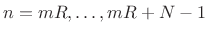
The sum over
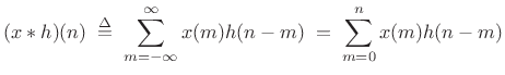
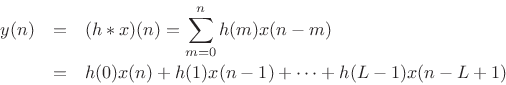
Convolution of Short Signals
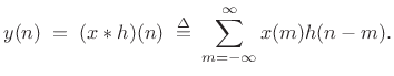
Figure 8.1 illustrates the conceptual operation of filtering an input
signal ![]() by a filter with impulse-response
by a filter with impulse-response ![]() to produce an
output signal
to produce an
output signal ![]() . By the convolution theorem for DTFTs
(§2.3.5),
. By the convolution theorem for DTFTs
(§2.3.5),
| (9.9) |
or,
| (9.10) |
where
 |
(9.11) |
In practice, we always use the DFT (preferably an FFT) in place of the DTFT, in which case we may write
| (9.12) |
where now
where
Another way to look at convolution is as the inner product of ![]() , and
, and
![]() , where
, where
![]() , i.e.,
, i.e.,
| (9.14) |
This form describes graphical convolution in which the output sample at time
Cyclic FFT Convolution
Thanks to the convolution theorem, we have two alternate ways to perform cyclic convolution in practice:
- Direct calculation in the time domain using (8.13)
- Frequency-domain convolution:
- Fourier Transform both signals
- Perform term by term multiplication of the transformed signals
- Inverse transform the result to get back to the time domain
Acyclic FFT Convolution
If we add enough trailing zeros to the signals being convolved, we can
obtain acyclic convolution embedded within a cyclic
convolution. How many zeros do we need to add? Suppose the signal
![]() consists of
consists of ![]() contiguous nonzero samples at times 0
to
contiguous nonzero samples at times 0
to
![]() , preceded and followed by zeros, and suppose
, preceded and followed by zeros, and suppose ![]() is nonzero
only over a block of
is nonzero
only over a block of ![]() samples starting at time 0. Then the
acyclic convolution of
samples starting at time 0. Then the
acyclic convolution of ![]() with
with ![]() reduces to
reduces to
 |
(9.15) |
which is zero for
The number
| (9.16) |
and so on.
When ![]() or
or ![]() is infinity, the convolution result can be as
small as 1. For example, consider
is infinity, the convolution result can be as
small as 1. For example, consider
![]() , with
, with
![]() , and
, and
![]() . Then
. Then
![]() . This is an example of what is called deconvolution.
In the frequency domain, deconvolution always involves a pole-zero
cancellation. Therefore, it is only possible when
. This is an example of what is called deconvolution.
In the frequency domain, deconvolution always involves a pole-zero
cancellation. Therefore, it is only possible when ![]() or
or ![]() is
infinite. In practice, deconvolution can sometimes be accomplished
approximately, particularly within narrow frequency bands
[119].
is
infinite. In practice, deconvolution can sometimes be accomplished
approximately, particularly within narrow frequency bands
[119].
We thus conclude that, to embed acyclic convolution within a cyclic
convolution (as provided by an FFT), we need to zero-pad both
operands out to length ![]() , where
, where ![]() is at least the sum of the
operand lengths (minus one).
is at least the sum of the
operand lengths (minus one).
Acyclic Convolution in Matlab
In Matlab or Octave, the conv function implements acyclic convolution:
octave:1> conv([1 2],[3 4])
ans =
   3  10   8
Note that it returns an output vector which is long enough to accommodate the entire result of the convolution, unlike the filter primitive, which always returns an output signal equal in length to the input signal:
octave:2> filter([1 2],1,[3 4])
ans =
   3  10
octave:3> filter([1 2],1,[3 4 0])
ans =
   3  10   8
Pictorial View of Acyclic Convolution
![\includegraphics[width=\textwidth ]{eps/convwaves}](http://www.dsprelated.com/josimages_new/sasp2/img1344.png)
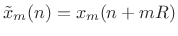
Figure 8.2 shows schematically the result of convolving
two zero-padded signals ![]() and
and ![]() . In this case, the signal
. In this case, the signal ![]() starts some time after
starts some time after ![]() , say at
, say at ![]() . Since
. Since ![]() begins at
time 0
, the output starts promptly at time
begins at
time 0
, the output starts promptly at time ![]() , but it takes some
time to ``ramp up'' to full amplitude. (This is the transient
response of the FIR filter
, but it takes some
time to ``ramp up'' to full amplitude. (This is the transient
response of the FIR filter ![]() .) If the length of
.) If the length of ![]() is
is ![]() , then
the transient response is finished at time
, then
the transient response is finished at time
![]() . Next, when
the input signal goes to zero at time
. Next, when
the input signal goes to zero at time ![]() , the output reaches
zero
, the output reaches
zero ![]() samples later (after the filter ``decay time''), or time
samples later (after the filter ``decay time''), or time
![]() . Thus, the total number of nonzero output samples is
. Thus, the total number of nonzero output samples is
![]() .
.
If we don't add enough zeros, some of our convolution terms ``wrap around'' and add back upon others (due to modulo indexing). This can be called time-domain aliasing. Zero-padding in the time domain results in more samples (closer spacing) in the frequency domain, i.e., a higher `sampling rate' in the frequency domain. If we have a high enough spectral sampling rate, we can avoid time aliasing.
The motivation for implementing acyclic convolution using a
zero-padded cyclic convolution is that we can use a Cooley-Tukey Fast Fourier
Transform (FFT) to implement cyclic convolution when its length ![]() is
a power of 2.
is
a power of 2.
Acyclic FFT Convolution in Matlab
The following example illustrates the implementation of acyclic convolution using a Cooley-Tukey FFT in matlab:
x = [1 2 3 4];
h = [1 1 1];

nx = length(x);
nh = length(h);
nfft = 2^nextpow2(nx+nh-1)
xzp = [x, zeros(1,nfft-nx)];
hzp = [h, zeros(1,nfft-nh)];
X = fft(xzp);
H = fft(hzp);

Y = H .* X;
format bank;
y = real(ifft(Y)) % zero-padded result
yt = y(1:nx+nh-1) % trim and print
yc = conv(x,h)    % for comparison
Program output:
nfft = 8
y =
  1.00  3.00  6.00  9.00  7.00  4.00  0.00  0.00
yt =
  1.00  3.00  6.00  9.00  7.00  4.00
yc =
     1     3     6     9     7     4
FFT versus Direct Convolution
Using the Matlab test program in
[264],9.1FFT convolution was found to be faster than direct convolution
starting at length ![]() (looking only at powers of 2 for the
length
(looking only at powers of 2 for the
length ![]() ).9.2 FFT convolution was also never
significantly slower at shorter lengths for which ``calling overhead''
dominates.
).9.2 FFT convolution was also never
significantly slower at shorter lengths for which ``calling overhead''
dominates.
Running the same test program in 2011,9.3 FFT convolution using the
fft function was found to be faster than conv for
all (power-of-2) lengths. The speed of FFT convolution divided
by that of direct convolution started out at 14 for ![]() , fell to a
minimum of
, fell to a
minimum of ![]() at
at ![]() , above which it started to climb as
expected, reaching
, above which it started to climb as
expected, reaching ![]() at
at
![]() . Note that this
comparison is unfair because the Octave fft function is a
dynamically linked, separately compiled module, while conv is
written in the matlab language and thus suffers more overhead from the
matlab interpreter.
. Note that this
comparison is unfair because the Octave fft function is a
dynamically linked, separately compiled module, while conv is
written in the matlab language and thus suffers more overhead from the
matlab interpreter.
An analysis reported in Strum and Kirk [279, p. 521],
based on the number of real multiplies, predicts that the fft
is faster starting at length ![]() , and that direct convolution is
significantly faster for very short convolutions (e.g., 16 operations
for a direct length-4 convolution, versus 176 for the fft
function).
, and that direct convolution is
significantly faster for very short convolutions (e.g., 16 operations
for a direct length-4 convolution, versus 176 for the fft
function).
See [264]9.4for further discussion of FFT algorithms and their applications.
In digital audio, FIR filters are often hundreds of taps long. For
such filters, the FFT method is much faster than direct convolution in
the time domain on single CPUs. On GPUs, FFT convolution is faster
than direct convolution only for much longer FIR-filter lengths (in
the thousands of taps [242]); this is because
massively parallel hardware can perform an
![]() algorithm
(direct convolution) faster than a single CPU can perform an
algorithm
(direct convolution) faster than a single CPU can perform an
![]() algorithm (FFT convolution).
algorithm (FFT convolution).
Audio FIR Filters
FIR filters shorter than the ear's ``integration time'' can generally be characterized by their magnitude frequency response (no perceivable ``delay effects''). The nominal ``integration time'' of the ear can be defined as the reciprocal of a critical bandwidth of hearing. Using Zwicker's definition of critical bandwidth [305], the smallest critical bandwidth of hearing is approximately 100 Hz (below 500 Hz). Thus, the nominal integration time of the ear is 10ms below 500 Hz. (Using the equivalent-rectangular-bandwidth (ERB) definition of critical bandwidth [179,269], longer values are obtained). At a 50 kHz sampling rate, this is 500 samples. Therefore, FIR filters shorter than the ear's ``integration time,'' i.e., perceptually ``instantaneous,'' can easily be hundreds of taps long (as discussed in the next section). FFT convolution is consequently an important implementation tool for FIR filters in digital audio applications.
Example 1: Low-Pass Filtering by FFT Convolution
In this example, we design and implement a length ![]() FIR lowpass
filter having a cut-off frequency at
FIR lowpass
filter having a cut-off frequency at ![]() Hz. The filter is
tested on an input signal
Hz. The filter is
tested on an input signal ![]() consisting of a sum of sinusoidal
components at frequencies
consisting of a sum of sinusoidal
components at frequencies
![]() Hz. We'll filter a
single input frame of length
Hz. We'll filter a
single input frame of length ![]() , which allows the FFT to be
, which allows the FFT to be
![]() samples (no wasted zero-padding).
samples (no wasted zero-padding).
% Signal parameters:
f = [ 440 880 1000 2000 ];      % frequencies
M = 256;                        % signal length
Fs = 5000;                      % sampling rate

% Generate a signal by adding up sinusoids:
x = zeros(1,M); % pre-allocate 'accumulator'
n = 0:(M-1);    % discrete-time grid
for fk = f;
    x = x + sin(2*pi*n*fk/Fs);
end
Next we design the lowpass filter using the window method:
% Filter parameters:
L = 257;    % filter length
fc = 600;   % cutoff frequency

% Design the filter using the window method:
hsupp = (-(L-1)/2:(L-1)/2);
hideal = (2*fc/Fs)*sinc(2*fc*hsupp/Fs);
h = hamming(L)' .* hideal; % h is our filter
![\includegraphics[width=\twidth]{eps/filter}](http://www.dsprelated.com/josimages_new/sasp2/img1365.png)
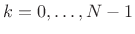
Figure 8.3 plots the impulse response and amplitude response of our FIR filter designed by the window method. Next, the signal frame and filter impulse response are zero-padded out to the FFT size and transformed:
% Choose the next power of 2 greater than L+M-1
Nfft = 2^(ceil(log2(L+M-1))); % or 2^nextpow2(L+M-1)

% Zero pad the signal and impulse response:
xzp = [ x zeros(1,Nfft-M) ];
hzp = [ h zeros(1,Nfft-L) ];

X = fft(xzp); % signal
H = fft(hzp); % filter
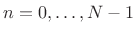
Figure 8.4 shows the input signal spectrum and the filter amplitude response overlaid. We see that only one sinusoidal component falls within the pass-band.
![\includegraphics[width=\twidth,height=1.8in]{eps/signal_transform}](http://www.dsprelated.com/josimages_new/sasp2/img1366.png)
![\includegraphics[width=\twidth,height=1.8in]{eps/filtered_transform}](http://www.dsprelated.com/josimages_new/sasp2/img1367.png) |
Now we perform cyclic convolution in the time domain using pointwise multiplication in the frequency domain:
Y = X .* H;The modified spectrum is shown in Fig.8.5.
The final acyclic convolution is the inverse transform of the pointwise product in the frequency domain. The imaginary part is not quite zero as it should be due to finite numerical precision:
y = ifft(Y);
relrmserr = norm(imag(y))/norm(y) % check... should be zero
y = real(y);
![\includegraphics[width=\twidth]{eps/filteredSignalAnn}](http://www.dsprelated.com/josimages_new/sasp2/img1368.png) |
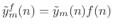
Figure 8.6 shows the filter output signal in the time domain. As expected, it looks like a pure tone in steady state. Note the equal amounts of ``pre-ringing'' and ``post-ringing'' due to the use of a linear-phase FIR filter.9.5
For an input signal approximately ![]() samples long, this example is
2-3 times faster than the conv function in Matlab (which is
precompiled C code implementing time-domain convolution).
samples long, this example is
2-3 times faster than the conv function in Matlab (which is
precompiled C code implementing time-domain convolution).
Example 2: Time Domain Aliasing
Figure 8.7 shows the effect of insufficient zero padding, which can be thought of as undersampling in the frequency domain. We will see aliasing in the time domain results.
The lowpass filter length is ![]() and the input signal consists of
an impulse at times
and the input signal consists of
an impulse at times ![]() and
and
![]() , where the data frame
length is
, where the data frame
length is ![]() . To avoid time aliasing (i.e., to implement
acyclic convolution using an FFT), we must use an FFT size
. To avoid time aliasing (i.e., to implement
acyclic convolution using an FFT), we must use an FFT size ![]() at
least as large as
at
least as large as
![]() . In the figure, the FFT sizes
. In the figure, the FFT sizes ![]() ,
,
![]() , and
, and ![]() are used. Thus, the first case is heavily time
aliased, the second only slightly time aliased (involving only some of
the filter's ``ringing'' after the second pulse), and the third is
free of time aliasing altogether.
are used. Thus, the first case is heavily time
aliased, the second only slightly time aliased (involving only some of
the filter's ``ringing'' after the second pulse), and the third is
free of time aliasing altogether.
![\includegraphics[width=\twidth]{eps/badoverlap}](http://www.dsprelated.com/josimages_new/sasp2/img1378.png) |
Convolving with Long Signals
We saw that we can perform efficient convolution of two finite-length sequences using a Fast Fourier Transform (FFT). There are some situations, however, in which it is impractical to use a single FFT for each convolution operand:
- One or both of the signals being convolved is very long.
- The filter must operate in real time. (We can't wait until the input signal ends before providing an output signal.)
Thus, at every time ![]() , the output
, the output ![]() can be computed as a linear
combination of the current input sample
can be computed as a linear
combination of the current input sample ![]() and the current filter
state
and the current filter
state
![]() .
.
To obtain the benefit of high-speed FFT convolution when the input
signal is very long, we simply chop up the input signal ![]() into
blocks, and perform convolution on each block separately. The output
is then the sum of the separately filtered blocks. The blocks
overlap because of the ``ringing'' of the filter. For a
zero-phase filter, each block overlaps with both of its neighboring
blocks. For causal filters, each block overlaps only with its
neighbor to the right (the next block in time). The fact that signal
blocks overlap and must be added together (instead of simply abutted)
is the source of the name overlap-add method for FFT
convolution of long sequences [7,9].
into
blocks, and perform convolution on each block separately. The output
is then the sum of the separately filtered blocks. The blocks
overlap because of the ``ringing'' of the filter. For a
zero-phase filter, each block overlaps with both of its neighboring
blocks. For causal filters, each block overlaps only with its
neighbor to the right (the next block in time). The fact that signal
blocks overlap and must be added together (instead of simply abutted)
is the source of the name overlap-add method for FFT
convolution of long sequences [7,9].
The idea of processing input blocks separately can be extended also to
both operands of a convolution (both ![]() and
and ![]() in
in ![]() ). The
details are a straightforward extension of the single-block-signal
case discussed below.
). The
details are a straightforward extension of the single-block-signal
case discussed below.
When simple FFT convolution is being performed between a signal ![]() and FIR filter
and FIR filter ![]() , there is no reason to use a non-rectangular
window function on each input block. A rectangular window
length of
, there is no reason to use a non-rectangular
window function on each input block. A rectangular window
length of ![]() samples may advance
samples may advance ![]() samples for each successive
frame (hop size
samples for each successive
frame (hop size ![]() samples). In this case, the input blocks do not
overlap, while the output blocks overlap by the FIR filter length
(minus one sample). On the other hand, if nonlinear and/or time-varying
spectral modifications to be performed, then there are good reasons to
use a non-rectangular window function and a smaller hop size, as we
will develop below.
samples). In this case, the input blocks do not
overlap, while the output blocks overlap by the FIR filter length
(minus one sample). On the other hand, if nonlinear and/or time-varying
spectral modifications to be performed, then there are good reasons to
use a non-rectangular window function and a smaller hop size, as we
will develop below.
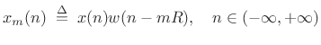
Overlap-Add Decomposition
Consider breaking an input signal ![]() into frames using a finite,
zero-phase, length
into frames using a finite,
zero-phase, length ![]() window
window ![]() . Then we may express the
. Then we may express the ![]() th
windowed data frame as
th
windowed data frame as
 |
(9.17) |
or
 |
(9.18) |
where

The hop size is the number of samples between the begin-times of adjacent frames. Specifically, it is the number of samples by which we advance each successive window.
Figure 8.8 shows an input signal (top) and three successive
windowed data frames using a length ![]() causal Hamming window and
50% overlap (
causal Hamming window and
50% overlap (![]() ).
).
![\includegraphics[width=\textwidth ]{eps/windsig}](http://www.dsprelated.com/josimages_new/sasp2/img1388.png)
For frame-by-frame spectral processing to work, we must be able to
reconstruct ![]() from the individual overlapping frames, ideally by
simply summing them in their original time positions. This can be
written as
from the individual overlapping frames, ideally by
simply summing them in their original time positions. This can be
written as
Hence,
![]() if and only if
if and only if
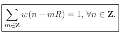 |
(9.19) |
This is the constant-overlap-add (COLA)9.6 constraint for the FFT analysis window
![\includegraphics[width=3.5in]{eps/cola}](http://www.dsprelated.com/josimages_new/sasp2/img1392.png)
Figure 8.9 illustrates the appearance of 50% overlap-add for
the Bartlett (triangular) window. The Bartlett window is clearly COLA
for a wide variety of hop sizes, such as ![]() ,
, ![]() , and so on,
provided
, and so on,
provided ![]() is an integer (otherwise the underlying continuous
triangular window must be resampled). However, when using windows
defined in a library, the COLA condition should be carefully checked.
For example, the following Matlab/Octave script shows that there
is a problem with the standard Hamming window:
is an integer (otherwise the underlying continuous
triangular window must be resampled). However, when using windows
defined in a library, the COLA condition should be carefully checked.
For example, the following Matlab/Octave script shows that there
is a problem with the standard Hamming window:
M = 33;          % window length
R = (M-1)/2;     % hop size
N = 3*M;         % overlap-add span
w = hamming(M);  % window
z = zeros(N,1);  plot(z,'-k');  hold on;  s = z;
for so=0:R:N-M
  ndx = so+1:so+M;        % current window location
  s(ndx) = s(ndx) + w;    % window overlap-add
  wzp = z; wzp(ndx) = w;  % for plot only
  plot(wzp,'--ok');       % plot just this window
end
plot(s,'ok');  hold off;  % plot window overlap-add
The figure produced by this matlab code is shown in Fig.8.10. As can be seen, the equal end-points sum to form an impulse in each frame of the overlap-add.
![\includegraphics[width=3.5in]{eps/tolaq}](http://www.dsprelated.com/josimages_new/sasp2/img1395.png)
The Matlab window functions (such as hamming) have an optional second argument which can be either 'symmetric' (the default), or 'periodic'. The periodic case is equivalent to
w = hamming(M+1); % symmetric case
w = w(1:M);       % delete last sample for periodic case
The periodic variant solves the non-constant overlap-add problem for even
w = hamming(M); % symmetric case
w(1) = w(1)/2;  % repair constant-overlap-add for R=(M-1)/2
w(M) = w(M)/2;
Since different window types may add or subtract 1 to/from
- hamming(M)

.54 - .46*cos(2*pi*(0:M-1)'/(M-1));
gives constant overlap-add for ,
,  , etc.,
when endpoints are divided by 2 or one endpoint is zeroed
, etc.,
when endpoints are divided by 2 or one endpoint is zeroed
- hanning(M)
.5*(1 - cos(2*pi*(1:M)'/(M+1)));
does not give constant overlap-add for
,
but does for 
- blackman(M)
.42 - .5*cos(2*pi*m)' + .08*cos(4*pi*m)';
where m = (0:M-1)/(M-1), gives constant overlap-add for when
when  is odd and
  is an integer, and
  when
is even and
is integer.
when
is even and
is integer.
In summary, all windows obeying the constant-overlap-add constraint
will yield perfect reconstruction of the original signal ![]() from the
data frames
from the
data frames
![]() by overlap-add (OLA). There
is no constraint on window type, only that the window overlap-adds to
a constant for the hop size used. In particular,
by overlap-add (OLA). There
is no constraint on window type, only that the window overlap-adds to
a constant for the hop size used. In particular, ![]() always yields
a constant overlap-add for any window function. We will learn later
(§8.3.1) that there is also a simple frequency-domain test on
the window transform for the constant overlap-add property.
always yields
a constant overlap-add for any window function. We will learn later
(§8.3.1) that there is also a simple frequency-domain test on
the window transform for the constant overlap-add property.
To emphasize an earlier point, if simple time-invariant FIR filtering
is being implemented, and we don't need to work with the intermediate
STFT, it is most efficient to use the rectangular window with
hop size ![]() , and to set
, and to set ![]() , where
, where ![]() is the length of the
filter
is the length of the
filter ![]() and
and ![]() is a convenient FFT size. The optimum
is a convenient FFT size. The optimum ![]() for a
given
for a
given ![]() is an interesting exercise to work out.
is an interesting exercise to work out.
COLA Examples
So far we've seen the following constant-overlap-add examples:
- Rectangular window at 0% overlap (hop size
= window size
)
- Bartlett window at 50% overlap (
 )
(Since normally
is odd, ``
'' means ``R=(M-1)/2,''
etc.)
)
(Since normally
is odd, ``
'' means ``R=(M-1)/2,''
etc.)
- Hamming window at 50% overlap (
)
- Rectangular window at 50% overlap (
)
- Hamming window at 75% overlap (
 % hop size)
- Any member of the Generalized Hamming family at 50% overlap
- Any member of the Blackman family at 2/3 overlap (1/3 hop size);
e.g., blackman(33,'periodic'),

- Any member of the
 -term Blackman-Harris family with
 .
.
- Any window with R=1 (``sliding FFT'')
STFT of COLA Decomposition
To represent practical FFT implementations, it is preferable
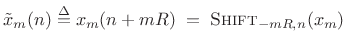
to shift the ![]() frame back to the time origin:
frame back to the time origin:
 |
(9.20) |
This is summarized in Fig.8.11. Zero-based frames are needed because the leftmost input sample is assigned to time zero by FFT algorithms. In other words, a hopping FFT effectively redefines time zero on each hop. Thus, a practical STFT is a sequence of FFTs of the zero-based frames
![\begin{psfrags}
% latex2html id marker 21934\psfrag{x}{$x$}\psfrag{Zero-centered 3rd frame x_3: M = 64, R = M/2}%
{\normalsize Zero-centered 3rd frame $x_3$: $M = 64$, $R = M/2$}\psfrag{x_3}{$x_3$} % doesn't work\psfrag{xtilde_3}{${\tilde x}_3$}\begin{figure}[htbp]
\includegraphics[width=\twidth]{eps/shiftwin}
\caption{Input signal $x$\ (top), third frame
$x_3$\ in its natural time location (middle), and the third frame
shifted to time 0, ${\tilde x}_3$\ (bottom).}
\end{figure}
\end{psfrags}](http://www.dsprelated.com/josimages_new/sasp2/img1412.png)
Note that we may sample the DTFT of both ![]() and
and
![]() ,
because both are time-limited to
,
because both are time-limited to ![]() nonzero samples. The
minimum information-preserving sampling interval along the unit circle
in both cases is
nonzero samples. The
minimum information-preserving sampling interval along the unit circle
in both cases is
![]() . In practice, we often
oversample to some extent, using
. In practice, we often
oversample to some extent, using ![]() with
with ![]() instead. For
instead. For
![]() , we get
, we get
where
 . For
. For
Since
![]() , their transforms are related by the
shift theorem:
, their transforms are related by the
shift theorem:

where ![]() denotes modulo
denotes modulo ![]() indexing (appropriate since the
DTFTs have been sampled at intervals of
indexing (appropriate since the
DTFTs have been sampled at intervals of
![]() ).
).
Acyclic Convolution
Getting back to acyclic convolution, we may write it as
Since
![]() is time limited to
is time limited to
![]() (or
(or
![]() ),
),
![]() can be sampled at intervals of
can be sampled at intervals of
![]() without time aliasing. If
without time aliasing. If ![]() is time-limited to
is time-limited to
![]() , then
, then
![]() will be time limited to
will be time limited to ![]() . Therefore, we may sample
. Therefore, we may sample
![]() at intervals of
at intervals of
 |
(9.22) |
or less along the unit circle. This is the dual of the usual sampling theorem.
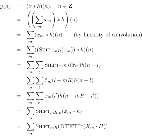
We conclude that practical FFT acyclic convolution may be carried out
using an FFT of any length ![]() satisfying
satisfying
| (9.23) |
where
![\begin{eqnarray*}
y(n) &=&
\sum_m \hbox{\sc Shift}_{mR,n} \left[\frac{1}{N} \sum_{k=0}^{N-1}
{\tilde H}(\omega_k) {\tilde X}_m(\omega_k) e^{j\omega_k n T}\right]\\
&=&
\sum_m \hbox{\sc Shift}_{mR,n}\left\{ \hbox{\sc IFFT}_N[\hbox{\sc FFT}_N({\tilde x}_m)\cdot \hbox{\sc FFT}_N(h)]\right\},
\end{eqnarray*}](http://www.dsprelated.com/josimages_new/sasp2/img1434.png)
where
![]() is the length
is the length ![]() DFT of the zero-padded
DFT of the zero-padded
![]() frame
frame
![]() , and
, and
![]() is the length
is the length ![]() DFT of
DFT of ![]() ,
also zero-padded out to length
,
also zero-padded out to length ![]() , with
, with
![]() .
.
Note that the terms in the outer sum overlap when ![]() even if
even if
![]() . In general, an LTI filtering by
. In general, an LTI filtering by ![]() increases
the amount of overlap among the frames.
increases
the amount of overlap among the frames.
This completes our derivation of FFT convolution between an
indefinitely long signal ![]() and a reasonably short FIR filter
and a reasonably short FIR filter
![]() (short enough that its zero-padded DFT can be practically
computed using one FFT).
(short enough that its zero-padded DFT can be practically
computed using one FFT).
The fast-convolution processor we have derived is a special case of the Overlap-Add (OLA) method for short-time Fourier analysis, modification, and resynthesis. See [7,9] for more details.
Example of Overlap-Add Convolution
Let's look now at a specific example of FFT convolution:
- Impulse-train test signal, 4000 Hz sampling-rate
- Length
 causal lowpass filter, 600 Hz cut-off
- Length
 rectangular window
- Hop size
 (no overlap)
We will work through the matlab for this example and display the results. First, the simulation parameters:
L = 31;         % FIR filter length in taps
fc = 600;       % lowpass cutoff frequency in Hz
fs = 4000;      % sampling rate in Hz

Nsig = 150;     % signal length in samples
period = round(L/3); % signal period in samples
FFT processing parameters:
M = L;                  % nominal window length
Nfft = 2^(ceil(log2(M+L-1))); % FFT Length
M = Nfft-L+1            % efficient window length
R = M;                  % hop size for rectangular window
Nframes = 1+floor((Nsig-M)/R);  % no. complete frames
Generate the impulse-train test signal:
sig = zeros(1,Nsig);
sig(1:period:Nsig) = ones(size(1:period:Nsig));
Design the lowpass filter using the window method:
epsilon = .0001;     % avoids 0 / 0
nfilt = (-(L-1)/2:(L-1)/2) + epsilon;
hideal = sin(2*pi*fc*nfilt/fs) ./ (pi*nfilt);
w = hamming(L); % FIR filter design by window method
h = w' .* hideal; % window the ideal impulse response

hzp = [h zeros(1,Nfft-L)];  % zero-pad h to FFT size
H = fft(hzp);               % filter frequency response
Carry out the overlap-add FFT processing:
y = zeros(1,Nsig + Nfft); % allocate output+'ringing' vector
for m = 0:(Nframes-1)
    index = m*R+1:min(m*R+M,Nsig); % indices for the mth frame
    xm = sig(index);  % windowed mth frame (rectangular window)
    xmzp = [xm zeros(1,Nfft-length(xm))]; % zero pad the signal
    Xm = fft(xmzp);
    Ym = Xm .* H;               % freq domain multiplication
    ym = real(ifft(Ym))         % inverse transform
    outindex = m*R+1:(m*R+Nfft);
    y(outindex) = y(outindex) + ym; % overlap add
end
The time waveforms for the first three frames (![]() ) are shown in
Figures 8.12 through 8.14. Notice how the causal linear-phase filtering results
in an overall signal delay by half the filter length. Also, note how
frames 0 and 2 contain four impulses, while frame 1 only happens to
catch three; this causes no difficulty, and the filtered result remains
correct by superposition.
) are shown in
Figures 8.12 through 8.14. Notice how the causal linear-phase filtering results
in an overall signal delay by half the filter length. Also, note how
frames 0 and 2 contain four impulses, while frame 1 only happens to
catch three; this causes no difficulty, and the filtered result remains
correct by superposition.
![\includegraphics[width=0.8\twidth]{eps/ola0}](http://www.dsprelated.com/josimages_new/sasp2/img1443.png)
![\includegraphics[width=0.8\twidth]{eps/ola1}](http://www.dsprelated.com/josimages_new/sasp2/img1444.png)
![\includegraphics[width=0.8\twidth]{eps/ola2}](http://www.dsprelated.com/josimages_new/sasp2/img1445.png)
Summary of Overlap-Add FFT Processing
Overlap-add FFT processors provide efficient implementations for FIR filters longer than 100 or so taps on single CPUs. Specifically, we ended up with:
![$\displaystyle y = \sum_{m=-\infty}^\infty \hbox{\sc Shift}_{mR} \left( \hbox{\sc DFT}_N^{-1} \left\{ H \cdot \hbox{\sc DFT}_N\left[\hbox{\sc Shift}_{-mR}(x)\cdot w \right]\right\}\right)$](http://www.dsprelated.com/josimages_new/sasp2/img1446.png) |
(9.24) |
where
- (1)
- Extract the
 th length
frame of data at time
th length
frame of data at time  .
.
- (2)
- Shift it to the base time interval
![$ [0,M-1]$](http://www.dsprelated.com/josimages_new/sasp2/img1448.png) (or
(or
![$ [-(M-1)/2,(M-1)/2]$](http://www.dsprelated.com/josimages_new/sasp2/img1426.png) ).
).
- (3)
- Optionally apply a length
analysis window
 (causal or zero phase, as preferred). For simple LTI filtering,
the rectangular window is fine.
(causal or zero phase, as preferred). For simple LTI filtering,
the rectangular window is fine.
- (4)
- Zero-pad the windowed data out to the FFT size
 (a power of 2),
such that
(a power of 2),
such that
 , where
is the FIR filter length.
, where
is the FIR filter length.
- (5)
- Take the
-point FFT.
- (6)
- Apply the filter frequency-response
 as a
windowing operation in the frequency domain.
as a
windowing operation in the frequency domain.
- (7)
- Take the
-point inverse FFT.
- (8)
- Shift the origin of the
-point result out to sample
where it belongs.
- (9)
- Sum into the output buffer containing the results from prior frames (OLA step).
A second condition is that the analysis window be COLA at the hop size used:
 |
(9.25) |
Dual of Constant Overlap-Add
In this section, we will derive the Fourier dual of the
Constant OverLap-Add (COLA) condition for STFT analysis windows
(discussed in §7.1). Recall that for perfect reconstruction
using a hop-size of ![]() samples, the window must be
samples, the window must be
![]() . We
will find that the equivalent frequency-domain condition is that the
window transform must have spectral zeros at all frequencies
which are a nonzero multiple of
. We
will find that the equivalent frequency-domain condition is that the
window transform must have spectral zeros at all frequencies
which are a nonzero multiple of ![]() . Following established
nomenclature for filter banks, we will say that such a window
transform is
. Following established
nomenclature for filter banks, we will say that such a window
transform is
![]() .
.
Poisson Summation Formula
Consider the summation of N complex sinusoids having frequencies uniformly spaced around the unit circle [264]:
![\begin{eqnarray*}
x(n) &\mathrel{\stackrel{\Delta}{=}}& \frac{1}{N} \sum_{k=0}^{N-1}e^{j\omega_kn} =
\left\{
\begin{array}{ll}
1 & n=0 \quad (\hbox{\sc mod}\ N) \\
0 & \mbox{elsewhere} \\
\end{array} \right. \\ [5pt]
&=& \hbox{\sc IDFT}_n(1 \cdots 1)
\end{eqnarray*}](http://www.dsprelated.com/josimages_new/sasp2/img1454.png)
where
 .
.
![\begin{psfrags}
% latex2html id marker 22700\psfrag{d(n)}{\normalsize $\displaystyle\normalsize \sum_l\delta(n-lN)$\ }\psfrag{\makebox[0pt][l]{2}N}{\normalsize $-2N$}\psfrag{\makebox[0pt][l]{N}}{\normalsize $-N$}\psfrag{0}{\normalsize $0$}\psfrag{N}{\normalsize $N$}\psfrag{n}{\normalsize $n$}\psfrag{2N}{\normalsize $2N$}\psfrag{1}{\normalsize $1$}\begin{figure}[htbp]
\includegraphics[width=3.5in]{eps/delta}
\caption{Discrete-time impulse train created
by a sum of sampled complex sinusoids.}
\end{figure}
\end{psfrags}](http://www.dsprelated.com/josimages_new/sasp2/img1456.png)
Setting ![]() (the FFT hop size) gives
(the FFT hop size) gives
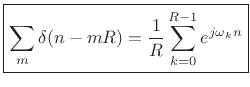 |
(9.26) |
where
 (harmonics of the frame rate).
Let us now consider these equivalent signals as inputs to an LTI
system, with an impulse response given by ![]() , and frequency response
equal to
, and frequency response
equal to ![]() .
.
![\begin{psfrags}
% latex2html id marker 22729\psfrag{w(n)}{\normalsize $w(n)$\ }\psfrag{W(w)}{\normalsize $W(\omega)$\ }\psfrag{timesum}{\normalsize $\displaystyle\sum_l\delta(n-lR)$\ }\psfrag{freqsum}{\normalsize $\frac{1}{R}\displaystyle\sum_k e^{j\omega_kn}$\ }\psfrag{t}{\normalsize $\displaystyle\sum_l w(n-lR)$\ }\psfrag{f}{\normalsize $\frac{1}{R}\displaystyle\sum_k W(\omega_k)e^{j\omega_kn}$\ }\psfrag{time}{\normalsize Time}\psfrag{freq}{\normalsize Frequency}\begin{figure}[htbp]
\includegraphics[width=4in]{eps/poisson}
\caption{Linear systems theory proof of the Poisson summation formula.}
\end{figure}
\end{psfrags}](http://www.dsprelated.com/josimages_new/sasp2/img1460.png)
Looking across the top of Fig.8.16, for the case of input signal
![]() we have
we have
 |
(9.27) |
Looking across the bottom of the figure, for the case of input signal
 |
(9.28) |
we have the output signal
 |
(9.29) |
This second form follows from the fact that complex sinusoids
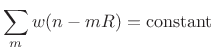
Since the inputs were equal, the corresponding outputs must be equal too. This derives the Poisson Summation Formula (PSF):
Note that the PSF is the Fourier dual of the sampling theorem [270], [264, Appendix G].
The continuous-time PSF is derived in §B.15.
Frequency-Domain COLA Constraints
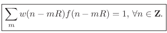
Recall that for error-free OLA processing, we required the constant-overlap-add (COLA) window constraint:
 |
(9.31) |
Thanks to the PSF, we may now express the COLA constraint in the frequency domain:
| (9.32) |
In other terms,

Notation:
The ``Nyquist(
We may also refer to (8.33) as the ``weak COLA constraint'' in the frequency domain. It gives necessary and sufficient conditions for perfect reconstruction in overlap-add FFT processors. However, when the short-time spectrum is being modified, these conditions no longer apply, and a stronger COLA constraint is preferable.
Strong COLA
An overly strong (but sufficient) condition is to require that
the window transform ![]() be bandlimited consistent with
downsampling by
be bandlimited consistent with
downsampling by ![]() :
:
This condition is sufficient, but not necessary, for perfect OLA reconstruction. Strong COLA implies weak COLA, but it cannot be achieved exactly by finite-duration window functions.
When either of the strong or weak COLA conditions are met, we have
 |
(9.34) |
That is, the overlap-add of the window
PSF Dual and Graphical Equalizers
Above, we used the Poisson Summation Formula to show that the constant-overlap-add of a window in the time domain is equivalent to the condition that the window transform have zero-crossings at all harmonics of the frame rate. In this section, we look briefly at the dual case: If the window transform is COLA in the frequency domain, what is the corresponding property of the window in the time domain? As one should expect, being COLA in the frequency domain corresponds to having specific uniform zero-crossings in the time domain.
Bandpass filters that sum to a constant provides an ideal basis for a graphic equalizer. In such a filter bank, when all the ``sliders'' of the equalizer are set to the same level, the filter bank reduces to no filtering at all, as desired.
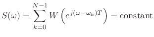
Let ![]() denote the number of (complex) filters in our filter bank,
with pass-bands uniformly distributed around the unit circle. (We will
be using an FFT to implement such a filter bank.) Denote the
frequency response of the ``dc channel'' by
denote the number of (complex) filters in our filter bank,
with pass-bands uniformly distributed around the unit circle. (We will
be using an FFT to implement such a filter bank.) Denote the
frequency response of the ``dc channel'' by
![]() . Then the
constant overlap-add property of the
. Then the
constant overlap-add property of the ![]() -channel filter bank can be
expressed as
-channel filter bank can be
expressed as
| (9.35) |
which means
 |
(9.36) |
where
 as usual. By the dual
of the Poisson summation formula, we have
as usual. By the dual
of the Poisson summation formula, we have
where
| (9.38) |
Thus, using the dual of the PSF, we have found that a good ![]() -channel
equalizer filter bank can be made using bandpass filters which have
zero-crossings at multiples of
-channel
equalizer filter bank can be made using bandpass filters which have
zero-crossings at multiples of ![]() samples, because that property
guarantees that the filter bank sums to a constant frequency response
when all channel gains are equal.
samples, because that property
guarantees that the filter bank sums to a constant frequency response
when all channel gains are equal.
The duality introduced in this section is the basis of the Filter-Bank Summation (FBS) interpretation of the short-time Fourier transform, and it is precisely the Fourier dual of the OverLap-Add (OLA) interpretation [9]. The FBS interpretation of the STFT is the subject of Chapter 9.
PSF and Weighted Overlap Add
Using ``square-root windows'' ![]() in the WOLA context, the
valid hop sizes
in the WOLA context, the
valid hop sizes ![]() are identical to those for
are identical to those for ![]() in the OLA case.
More generally, given any window
in the OLA case.
More generally, given any window ![]() for use in a WOLA system, it
is of interest to determine the hop sizes which yield perfect
reconstruction.
for use in a WOLA system, it
is of interest to determine the hop sizes which yield perfect
reconstruction.
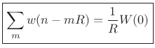
Recall that, by the Poisson Summation Formula (PSF),
![$\displaystyle \zbox {\underbrace{\sum_m w(n-mR)}_{\hbox{\sc Alias}_R(w)} = \underbrace{\frac{1}{R}\sum_{k=0}^{R-1} W(\omega_k)e^{j\omega_k n}}_{\hbox{\sc DFT}_R^{-1} \left[\hbox{\sc Sample}_{\frac{2\pi}{R}}(W)\right]}} \quad \omega_k \isdef \frac{2\pi k}{R} \protect$](http://www.dsprelated.com/josimages_new/sasp2/img1466.png) |
(9.39) |
For WOLA, this is easily modified to become
![$\displaystyle \zbox {\underbrace{\sum_m w(n-mR)f(n-mR)}_{\hbox{\sc Alias}_R(w\cdot f)} = \underbrace{\frac{1}{R}\sum_{k=0}^{R-1} (W\ast F)(\omega_k)e^{j\omega_k n}}_{\hbox{\sc DFT}_R^{-1} \left[\hbox{\sc Sample}_{\frac{2\pi}{R}}(W\ast F)\right]}} \quad \omega_k \isdef \frac{2\pi k}{R}$](http://www.dsprelated.com/josimages_new/sasp2/img1482.png) |
(9.40) |
where
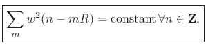
When ![]() , this becomes
, this becomes
![$\displaystyle \underbrace{\sum_m w^2(n-mR)}_{\hbox{\sc Alias}_R(w^2)} = \underbrace{\frac{1}{R}\sum_{k=0}^{R-1} (W\ast W)(\omega_k)e^{j\omega_k n}}_{\hbox{\sc DFT}_R^{-1} \left[\hbox{\sc Sample}_{\frac{2\pi}{R}}(W\ast W)\right]}, \quad \omega_k \isdef \frac{2\pi k}{R}$](http://www.dsprelated.com/josimages_new/sasp2/img1485.png) |
(9.41) |
Example COLA Windows for WOLA
In a weighted overlap-add system, the following windows can be used to satisfy the constant-overlap-add condition:
- For the rectangular window,
 , and
, and
 (since
 is a sinc function which reduces to
 when
when
 , and
, and
 .
.
- For the Hamming window, the critically sampled window transform
has three nonzero samples (where the rectangular-window transform has
one). Therefore,
 has
has  nonzero samples at critical
sampling. Measuring main-lobe width from zero-crossing to
zero-crossing as usual, we get
nonzero samples at critical
sampling. Measuring main-lobe width from zero-crossing to
zero-crossing as usual, we get
 radians per sample, or
``6 side lobes'', for the width of
.
radians per sample, or
``6 side lobes'', for the width of
.
- The squared-Blackman window transform width is
 .
.
- The square of a length
-term Blackman-Harris-family window
(where rect is
 , Hann is
  , etc.) has a main lobe of width
 , measured from zero-crossing to zero-crossing in
``side-lobe units'' (
, measured from zero-crossing to zero-crossing in
``side-lobe units'' ( ). This is up from
 for the
original
-term window.
for the
original
-term window.
- The width of the main lobe can be used to determine the
hop size in the STFT, as will be discussed further in
Chapter 9.
Note that we need only find the first zero-crossing in the
window transform for any member of the Blackman-Harris window family
(Chapter 3), since nulls at all harmonics of
that frequency will always be present (at multiples of ![]() ).
).
Overlap-Save Method
The classical overlap-save method [198,277], unlike OLA, uses no zero padding to prevent time aliasing. Instead, it
- (1)
- discards output samples corrupted by time aliasing each frame, and
- (2)
- overlaps the input frames by the same amount.
More specifically:
- If the input frame size is
and the filter
length is
 , then a length
FFT and IFFT are used.
, then a length
FFT and IFFT are used.
- As a result,
 samples of the output are invalid due to time aliasing.
- The overlap-save method writes out the good
 samples
and uses a hop size of
, thus recomputing the time-aliased output
samples in the previous frame.
samples
and uses a hop size of
, thus recomputing the time-aliased output
samples in the previous frame.
Time Varying OLA Modifications
In the preceding sections, we assumed that the spectral modification
![]() did not vary over time. We will now examine the implications of
time-varying spectral modifications. The derivation below
follows [9], except that we'll keep our previous
notation:
did not vary over time. We will now examine the implications of
time-varying spectral modifications. The derivation below
follows [9], except that we'll keep our previous
notation:
Using ![]() in our OLA formulation with a hop size
in our OLA formulation with a hop size ![]() results in
results in
![\begin{eqnarray*}
y(n) &=& \sum_{m=-\infty}^\infty y_m(n) \\
&=& \sum_{m=-\infty}^\infty \frac{1}{N}\sum_{k=0}^{N-1} X_m(\omega_k) H_m(\omega_k) e^{j\omega_kn} \\
&=& \sum_{m=-\infty}^\infty \frac{1}{N}\sum_{k=0}^{N-1}
\left[ \sum_{l=-\infty}^\infty x(l) w(l-m)e^{-j\omega_kl} \right]
H_m(\omega_k) e^{j\omega_kn} \\
&=& \sum_{l=-\infty}^\infty x(l) \sum_{m=-\infty}^\infty w(l-m)
\frac{1}{N}\sum_{k=0}^{N-1} H_m(\omega_k)
e^{j\omega_k(n-l)} \\
&=& \sum_{l=-\infty}^\infty x(l)
\sum_{m=-\infty}^\infty w(l-m) h_m(n-l) \\
\end{eqnarray*}](http://www.dsprelated.com/josimages_new/sasp2/img1499.png)
Define
 to get
 |
(9.42) |
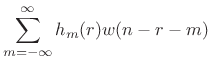
Let's examine the term
 in more detail:
 describes the time variation of the
  tap.
tap.
-
![$ \sum_{m=-\infty}^\infty h_m(r) w[(n-r)-m] = [h_{(\cdot)}(r) \ast w](n-r)$](http://www.dsprelated.com/josimages_new/sasp2/img1505.png) is a filtered version of the
tap
. It is
lowpass-filtered by w and delayed by
is a filtered version of the
tap
. It is
lowpass-filtered by w and delayed by  samples.
- Denote the
th time-varying, lowpass-filtered, delayed-by-
filter tap by
 . This can be interpreted
as the weighting in the output at time
of an impulse entering
the time-varying filter at time
. This can be interpreted
as the weighting in the output at time
of an impulse entering
the time-varying filter at time  .
.

This is a superposition sum for an arbitrary linear, time-varying filter
![]() .
.
Block Diagram Interpretation of Time-Varying STFT Modifications
Assuming ![]() is causal gives
is causal gives
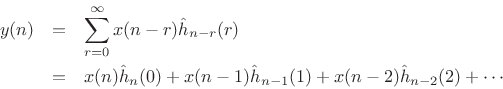
This is depicted in Fig.8.17.
![\begin{psfrags}
% latex2html id marker 23334\psfrag{zm1}{\large $z^{-1}$\ }\psfrag{h(0,n)}{\large$ h_n(0) $}\psfrag{h(1,n)}{\large$ h_{n-1}(1) $}\psfrag{h(2,n)}{\large$ h_{n-L+1}(L-1) $}\psfrag{+}{\large$\Sigma$}\psfrag{w(n)}{\large$ w $}\psfrag{y(n)}{\large$ y(n) $}\begin{figure}[htbp]
\includegraphics[width=\twidth]{eps/olamods}
\caption{System diagram giving
an interpretation of the bandlimited time-varying filter coefficients
in the overlap-add STFT processor with a new filter each frame.}
\end{figure}
\end{psfrags}](http://www.dsprelated.com/josimages_new/sasp2/img1511.png)
The term ![]() can be interpreted as the FIR filter tap
can be interpreted as the FIR filter tap ![]() at time
at time
![]() . Note how each tap is lowpass filtered by the FFT window
. Note how each tap is lowpass filtered by the FFT window
![]() . The window thus enforces bandlimiting each filter tap to
the bandwidth of the window's main lobe. For an
. The window thus enforces bandlimiting each filter tap to
the bandwidth of the window's main lobe. For an ![]() -term length-
-term length-![]() Blackman-Harris window, for example, the main-lobe reaches zero at
frequency
Blackman-Harris window, for example, the main-lobe reaches zero at
frequency
![]() (see Table 5.2 in §5.5.2
for other examples). This bandlimiting places a limit on the bandwidth expansion
caused by time-variation of the filter coefficients, which in turn places a limit
on the maximum STFT hop-size that can be used without frequency-domain aliasing.
See Allen and Rabiner 1977
[9] for further details on the bandlimiting
property.
(see Table 5.2 in §5.5.2
for other examples). This bandlimiting places a limit on the bandwidth expansion
caused by time-variation of the filter coefficients, which in turn places a limit
on the maximum STFT hop-size that can be used without frequency-domain aliasing.
See Allen and Rabiner 1977
[9] for further details on the bandlimiting
property.
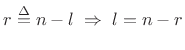
Length L FIR Frame Filters
To avoid time aliasing, we restrict the filter length to a maximum of
![]() samples. Since
samples. Since
![]() is an arbitrary multiplicative
weighting of the
is an arbitrary multiplicative
weighting of the ![]() th spectral frame, the frame filter need not be
causal. For odd
th spectral frame, the frame filter need not be
causal. For odd ![]() , the filter impulse response indices may run from
, the filter impulse response indices may run from
![]() to
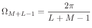
to ![]() , where
, where
 |
(9.43) |
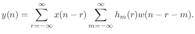
This gives
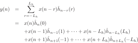
This is the general length ![]() time-varying FIR filter convolution sum for
time
time-varying FIR filter convolution sum for
time ![]() , when
, when ![]() is odd.
is odd.
Weighted Overlap Add
In the weighted overlap add (WOLA) method, we apply a second window after the inverse DFT [49] and prior to the final overlap-add to create the output signal. Such a window can be called a ``synthesis window,'' ``postwindow,'' or simply ``output window.''
Output windows are important in audio compression applications for minimizing ``blocking effects.'' The synthesis window ``fades out'' any spectral coding error at the frame boundaries, thereby suppressing audible discontinuities.
Output windows are not used in simple FFT convolution processors because the input frames are supposed to be expanded by the convolution, and a synthesis window would ``pinch off'' the ``filter ringing'' from each block, yielding incorrect results. Output windows can always be used in conjunction with spectral modifications made by means of the ``filter bank summation'' (FBS) method, which is the subject of the next chapter.
The WOLA method is most useful for nonlinear ``instantaneous'' FFT processors such as
- perceptual audio coders,
- time-scale modification, or
- pitch-shifters.
WOLA Processing Steps
The sequence of operations in a WOLA processor can be expressed as follows:
- Extract the
th windowed frame of data
 ,
,
 (assuming a length
  causal window
and hop
size
).
causal window
and hop
size
).
- Take an FFT of the
th frame translated to time zero,
 , to produce the
th spectral frame
, to produce the
th spectral frame
 ,
,
 .
.
- Process
as desired to produce
 .
.
- Inverse FFT
 to produce
 ,
,
 .
.
- Apply a synthesis window
 to
to yield a
weighted output frame
to
to yield a
weighted output frame
 ,
.
,
.
- Translate the
th output frame to time
as
 and add to the accumulated output signal
  .
.
To obtain perfect reconstruction in the absence of spectral modifications, we require
which is true if and only if
 |
(9.44) |
Choice of WOLA Window
The synthesis (output) window in weighted overlap-add is typically chosen to be the same as the analysis (input) window, in which case the COLA constraint becomes
 |
(9.45) |
We can say that
A trivial way to construct useful windows for WOLA is to take the
square root of any good OLA window. This works for all non-negative
OLA windows (which covers essentially all windows in Chapter 3
other than Portnoff windows). For example, the
``root-Hann window'' can be defined for odd ![]() by
by
Notice that the root-Hann window is the same thing as the ``MLT Sine Window'' described in §3.2.6. We can similarly define the ``root-Hamming'', ``root-Blackman'', and so on, all of which give perfect reconstruction in the weighted overlap-add context.
Review of Zero Padding
Expanding on the discussion in §2.5, zero-padding is used for
- Spectral interpolation
- -
- Clearer spectral magnitude/phase plots
- -
- Sinusoidal peak tracking (e.g., to help quadratic interpolation)
- To extend to the next highest power of 2 (FFT)
- To make room for ``filter ringing'' in overlap-add convolution using an FFT
Next Section:
The Filter Bank Summation (FBS) Interpretation of the Short Time Fourier Transform (STFT)
Previous Section:
Time-Frequency Displays


