


Time-Varying Delay Effects
In the category of delay effects, variable delay lines are used for
(While reverberators need not be time varying, nowadays they typically are [104,58].)In digital waveguide synthesis, variable delay lines are used for
- Vibrating strings (guitars, violins, ...)
- Woodwind bores
- Horns
- Tonal percussion (rods, membranes)
After an implementation note on time-varying delay lines, we will look at a number of time-varying delay effects requiring variable delay lines. The use of variable delay lines in digital waveguide models will be taken up Chapter 6.
Variable Delay Lines
Time varying delay lines are fundamental building blocks for delay effects, synthesis algorithms, and computational acoustic models of musical instruments.
Let A denote an array of length ![]() . Then we can implement an
. Then we can implement an
![]() -sample variable delay line in the C programming language
as shown in Fig.5.1. We require, of course,
-sample variable delay line in the C programming language
as shown in Fig.5.1. We require, of course, ![]() .
.
   static double A[N];
   static double *rptr = A; // read ptr
   static double *wptr = A; // write ptr

   double setdelay(int M) {
       rptr = wptr - M;
       while (rptr < A) { rptr += N }
   }

   double delayline(double x)
   {
     double y;
     A[wptr++] = x;
     y = A[rptr++];
     if ((wptr-A) >= N) { wptr -= N }
     if ((rptr-A) >= N) { rptr -= N }
     return y;
   }
|
The Synthesis Tool Kit, Version 4 [86] contains the C++ class ``Delay'' which implements this type of variable (but non-interpolating) delay line. There are additional subclasses which provide interpolating reads by various methods. In particular, the class DelayL implements continuously variable delay lengths using linear interpolation. The code listing in Fig.5.1 can be modified to use linear interpolation by replacing the line
y = A[rptr++];with
  long rpi = (long)floor(rptr);
  double a = rptr - (double)rpi;
  y = a * A[rpi] + (1-a) * A[rpi+1];
  rptr += 1;
To implement a continuously varying delay, we add a ``delay growth parameter'' g to the delayline function in Fig.5.1, and change the line
rptr += 1; // pointer updateabove to
rptr += 1 - g; // pointer updateWhen g is 0, we have a fixed delay line. When
Doubling and Slap-Back
The doubling effect is a studio recording technique often used to ``thicken'' vocals in which the same part is sung twice by the same person. In other words, doubling is a ``chorus of two'', where both parts are sung ``in unison'' by the same person. As an example, the Beatles used doubling very often, such as on the track ``Hard Day's Night''. A single variable delay line can simulate doubling very effectively.
The related term slap back refers to the use of a single echo on a recorded track. The echo is often placed in a different spatial location in the stereo mix. Normally the echo delay is just large enough to be heard as a discrete echo on careful listening (e.g., on the order of tens of milliseconds). Compared to doubling, slap back uses a larger delay relative to the first voice, and the delay need not vary.
Flanging
Flanging is a delay effect that has been available in recording studios since at least the 1960s. Surprisingly little literature exists, although there is some [32,429,59,17,104,242].6.1
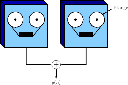
The term ``flanging'' is said to have arisen from the way the effect was originally achieved by two tape machines set up to play the same tape in unison, with their outputs added together (mixed equally), as shown in Fig.5.2. To achieve the flanging effect, the flange of one of the supply reels is touched lightly to make it play a littler slower. This causes a delay to develop between the two tape machines. The flange is released, and the flange of the other supply reel is touched lightly to slow it down. This causes the delay to gradually disappear and then begin to grow again in the opposite direction. The delay is kept below the threshold of echo perception (e.g., only a few milliseconds in each direction). The process is repeated as desired, pressing the flange of each supply reel in alternation. The flanging effect has been described as a kind of ``whoosh'' passing subtly through the sound.6.2The effect is also compared to the sound of a jet passing overhead, in which the direct signal and ground reflection arrive at a varying relative delay [59]. If flanging is done rapidly enough, an audible Doppler shift is introduced which approximates the ``Leslie'' effect commonly used for organs (see §5.9).
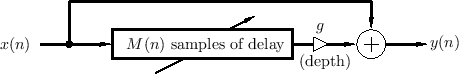
Flanging is modeled quite accurately as a feedforward comb filter, as
discussed in §2.6.1, in which the delay ![]() is varied
over time. Figure 5.3 depicts such a model. The input-output
relation for a basic flanger can be written as
is varied
over time. Figure 5.3 depicts such a model. The input-output
relation for a basic flanger can be written as
where
As shown in Fig.2.25, the frequency response of Eq.![]() (5.1)
has a ``comb'' shaped structure. For
(5.1)
has a ``comb'' shaped structure. For ![]() , there are
, there are ![]() peaks in the frequency response, centered about frequencies
peaks in the frequency response, centered about frequencies
As is evident from Fig.2.25, at any given time there are ![]() notches in the flanger's amplitude response (counting positive-
and negative-frequency notches separately). The notches are thus
spaced at intervals of
notches in the flanger's amplitude response (counting positive-
and negative-frequency notches separately). The notches are thus
spaced at intervals of ![]() Hz, where
Hz, where ![]() denotes the sampling
rate. In particular, the notch spacing is inversely
proportional to delay-line length.
denotes the sampling
rate. In particular, the notch spacing is inversely
proportional to delay-line length.
The time variation of the delay-line length ![]() results in a
``sweeping'' of uniformly-spaced notches in the spectrum. The
flanging effect is thus created by moving notches in the
spectrum. Notch motion is essential for the flanging effect. Static
notches provide some coloration to the sound, but an isolated notch
may be inaudible [139]. Since the steady-state sound
field inside an undamped acoustic tube has a similar set of
uniformly spaced notches (except at the ends), a static row of notches
tends to sound like being inside an acoustic tube.
results in a
``sweeping'' of uniformly-spaced notches in the spectrum. The
flanging effect is thus created by moving notches in the
spectrum. Notch motion is essential for the flanging effect. Static
notches provide some coloration to the sound, but an isolated notch
may be inaudible [139]. Since the steady-state sound
field inside an undamped acoustic tube has a similar set of
uniformly spaced notches (except at the ends), a static row of notches
tends to sound like being inside an acoustic tube.
Flanger Speed and Excursion
As mentioned above, the delay-line length ![]() in a digital flanger
is typically modulated by a low-frequency oscillator (LFO).
The oscillator waveform is usually triangular, sinusoidal, or
exponential (triangular on a log-frequency scale). In the sinusoidal
case, we have the following delay variation:
in a digital flanger
is typically modulated by a low-frequency oscillator (LFO).
The oscillator waveform is usually triangular, sinusoidal, or
exponential (triangular on a log-frequency scale). In the sinusoidal
case, we have the following delay variation:
Flanger Depth Control
To obtain a maximum effect, the depth control, ![]() in Fig.5.3,
should be set to 1. A depth of
in Fig.5.3,
should be set to 1. A depth of ![]() gives no effect.
gives no effect.
Flanger Inverted Mode
A different type of maximum depth is obtained for ![]() . In this
case, the peaks and notches of the
. In this
case, the peaks and notches of the ![]() case trade places. In
practice, the depth control
case trade places. In
practice, the depth control ![]() is usually constrained to the interval
is usually constrained to the interval
![]() , and a sign inversion for
, and a sign inversion for ![]() is controlled separately using a
``phase inversion'' switch.
is controlled separately using a
``phase inversion'' switch.
In inverted mode, unless the delay ![]() is very large, the bass
response will be weak, since the first notch is at dc. This case
usually sounds high-pass filtered relative to the ``in-phase'' case
(
is very large, the bass
response will be weak, since the first notch is at dc. This case
usually sounds high-pass filtered relative to the ``in-phase'' case
(![]() ).
).
As the notch spacing grows very large (![]() shrinks), the amplitude
response approaches that of a first-order difference
shrinks), the amplitude
response approaches that of a first-order difference
![]() , which approximates a differentiator
, which approximates a differentiator
![]() . An ideal differentiator eliminates dc and provides
a progressive high-frequency boost rising 6 dB per octave
(specifically, the amplitude response is
. An ideal differentiator eliminates dc and provides
a progressive high-frequency boost rising 6 dB per octave
(specifically, the amplitude response is
![]() ).
).
Flanger Feedback Control
Many modern commercial flangers have a control knob labeled ``feedback'' or ``regen.'' This control sets the level of feedback from the output to the input of the delay line, thereby creating a feedback comb filter in addition to the feedforward comb filter, in the same manner as in the creation of a Schroeder allpass filter in §2.8.1 (see Fig.2.30).
Summary of Flanging
In view of the above, we may define a flanger in general as any filter which modulates the frequencies of a set of uniformly spaced notches and/or peaks in the frequency response. The main parameters are
- Depth
![$ g\in[0,1]$](http://www.dsprelated.com/josimages_new/pasp/img1245.png) -- controlling notch depth
-- controlling notch depth
- Speed
 -- speed of notch movement
- Phase -- switch to subtract instead of adding the direct signal with the delayed signal
- Average Delay

- Excursion or Sweep
 -- amount by which the delay-line grows or shrinks
- Feedback or Regeneration
 -- feedback coefficient from output to input
Note that flanging provides only uniformly spaced notches.
This can be considered non-ideal for several reasons. First, the ear
processes sound over a frequency scale that is more nearly logarithmic
than linear [459]. Therefore, exponentially spaced
notches (uniformly spaced on a log frequency scale) should sound more
uniform perceptually. Secondly, the uniform peaks and notches of the
flanger can impose a discernible ``resonant pitch'' on the program
material, giving the impression of being inside a resonant tube.
Third, when ![]() (inverted flanging), it is possible for a periodic
tone to be completely annihilated by harmonically spaced notches if
the harmonics of the tone are unlucky enough to land exactly on a
subset of the harmonic notches. In practice, exact alignment is
unlikely; however, the signal loudness can be modulated to a possibly
undesirable degree as the notches move through alignment with the
signal spectrum. For this reason, flangers are best used with
noise-like or inharmonic sounds. For harmonic signals, it makes sense
to consider methods for creating non-uniform moving notches.
(inverted flanging), it is possible for a periodic
tone to be completely annihilated by harmonically spaced notches if
the harmonics of the tone are unlucky enough to land exactly on a
subset of the harmonic notches. In practice, exact alignment is
unlikely; however, the signal loudness can be modulated to a possibly
undesirable degree as the notches move through alignment with the
signal spectrum. For this reason, flangers are best used with
noise-like or inharmonic sounds. For harmonic signals, it makes sense
to consider methods for creating non-uniform moving notches.
A Faust software implementation of flanging may be found in the file effect.lib within the Faust distribution [154,170]. The Faust programming example phaser_flanger.dsp may be run to hear the effect on a test signal and experiment with its parameters in real time.
Phasing
The phaser, or phase shifter, is closely related to the flanger in that it also works by sweeping notches through the spectrum of the input signal. While the term phasing is sometimes used synonymously with flanging [32],6.4 typical commercial phase shifters have been observed to implement nonuniformly spaced notches.6.5 Furthermore, phasers such as the Univibe (1960s) were intended to simulate the Leslie rotating speaker effect (§5.9) as opposed to being a low-cost analog flanging approximation. In other words, the conceptual unification of phasing and flanging seems to be technical in nature; i.e., based on the fact that both effects operate by sweeping notches through the spectrum. Flangers are constrained to have an ``infinite series'' of harmonically spaced notches (§2.6.3), while phasers have a limited number of nonuniformly spaced notches. In both cases motion of the notches over time is essential to the effect, and this motion is classically periodic. We will therefore define a phaser as any linear filter which modulates the frequencies of a set of non-uniformly spaced notches, while a flanger will remain any device which modulates uniformly spaced notches.
Digital implementations of phase shifters are discussed in §8.9. A Faust phase-shifter may be found in the file effect.lib within the Faust software distribution [154,170]. The Faust programming example phaser_flanger.dsp demonstrates the phasing effect.
Vibrato Simulation
The term vibrato refers to small, quasi-periodic variations in
the pitch of a tone. On a violin, for example, vibrato is
produced by wiggling the finger stopping the string on the
fingerboard; a violin vibrato frequency can be very slow, or a bit
faster than 6 Hz. A typical vibrato depth is on the order of 1
percent (a semitone is
![]() percent). In the
singing voice, vibrato is produced by modulating the tension of the
vocal folds. Vibrato is typically accompanied by
tremolo, which is amplitude modulation at the same
frequency as the vibrato which causes it. For example, in the violin,
the frequency-modulations of the string vibrations are translated into
amplitude modulations by the complex variations in the frequency
response of the violin body.
percent). In the
singing voice, vibrato is produced by modulating the tension of the
vocal folds. Vibrato is typically accompanied by
tremolo, which is amplitude modulation at the same
frequency as the vibrato which causes it. For example, in the violin,
the frequency-modulations of the string vibrations are translated into
amplitude modulations by the complex variations in the frequency
response of the violin body.
To apply vibrato to a sound, it is necessary to apply a quasi-periodic frequency shift. This can be accomplish using a modulated delay line. This works because a time-varying delay line induces a simulated Doppler shift on the signal within it.
The flanger in effect.lib (Faust distribution) has a vibrato mode in which it becomes a pure time-varying delay line. This mode can be accessed via a checkbox in the example phaser_flanger.dsp.
Doppler Effect
The Doppler effect causes the pitch of a sound source to appear to rise or fall due to motion of the source and/or listener relative to each other. You have probably heard the pitch of a horn drop lower as it passes by (e.g., from a moving train). As a pitched sound-source moves toward you, the pitch you hear is raised; as it moves away from you, the pitch is lowered. The Doppler effect has been used to enhance the realism of simulated moving sound sources for compositional purposes [80], and it is an important component of the ``Leslie effect'' (described in §5.9).
As derived in elementary physics texts, the Doppler shift is given by
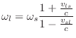
where
Vector Formulation
Denote the sound-source velocity by
![]() where
where
![]() is time. Similarly,
let
is time. Similarly,
let
![]() denote the velocity of the listener, if any. The
position of source and listener are denoted
denote the velocity of the listener, if any. The
position of source and listener are denoted
![]() and
and
![]() , respectively, where
, respectively, where
![]() is 3D
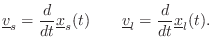
position. We have velocity related to position by
is 3D
position. We have velocity related to position by
Consider a Fourier component of the source at frequency
The Doppler effect depends only on velocity components along the line
connecting the source and listener [349, p. 453]. We may
therefore orthogonally project the source and listener
velocities onto the vector
![]() pointing from the source
to the listener. (See Fig.5.8 for a specific example.)
pointing from the source
to the listener. (See Fig.5.8 for a specific example.)
The orthogonal projection of a vector
![]() onto a vector
onto a vector
![]() is given by [451]
is given by [451]

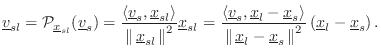
In the far field (listener far away), Eq.
Doppler Simulation
It is well known that a time-varying delay line results in a frequency shift. Time-varying delay is often used, for example, to provide vibrato and chorus effects [17]. We therefore expect a time-varying delay-line to be capable of precise Doppler simulation. This section discusses simulating the Doppler effect using a variable delay line [468].6.6
Consider Doppler shift from a physical point of view. The air can be
considered as analogous to a magnetic tape which moves from
source to listener at speed ![]() (see Fig.5.4). The source is
analogous to the
write-head of a tape recorder, and the listener corresponds to the
read-head. When the source and listener are fixed, the listener
receives what the source records. When either moves, a Doppler shift
is observed by the listener, according
to Eq.
(see Fig.5.4). The source is
analogous to the
write-head of a tape recorder, and the listener corresponds to the
read-head. When the source and listener are fixed, the listener
receives what the source records. When either moves, a Doppler shift
is observed by the listener, according
to Eq.![]() (5.2).6.7
(5.2).6.7

Doppler Simulation via Delay Lines
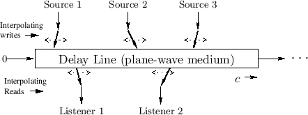
This analogy also works for a delay-line based computational model,
as depicted in Fig.5.5.
The magnetic tape is now the delay line, the tape read-head is the
read-pointer of the delay line, and the write-head is the delay-line
write-pointer. In this analogy, it is readily verified
that modulating delay by changing the read-pointer increment from 1 to
![]() (thereby requiring interpolated reads) corresponds to
listener motion away from the source at speed
(thereby requiring interpolated reads) corresponds to
listener motion away from the source at speed ![]() . It also follows
that changing the write-pointer increment from
. It also follows
that changing the write-pointer increment from ![]() to
to
![]() corresponds source motion toward the listener at
speed
corresponds source motion toward the listener at
speed ![]() .
When this is done, we must use interpolating writes into the
delay memory. Interpolating writes may be called
de-interpolation [502], and they are formally the
graph-theoretic transpose of interpolating reads (ordinary
``interpolation'') [333]. A review of
time-varying, interpolating, delay-line reads and writes, together
with a method using a single shared pointer, are given in
[383].
.
When this is done, we must use interpolating writes into the
delay memory. Interpolating writes may be called
de-interpolation [502], and they are formally the
graph-theoretic transpose of interpolating reads (ordinary
``interpolation'') [333]. A review of
time-varying, interpolating, delay-line reads and writes, together
with a method using a single shared pointer, are given in
[383].
Time-Varying Delay-Line Reads
If ![]() denotes the input to a time-varying delay, the output can be
written as
denotes the input to a time-varying delay, the output can be
written as
Let's analyze the frequency shift caused by a time-varying delay by
setting ![]() to a complex sinusoid at frequency
to a complex sinusoid at frequency ![]() :
:
where
Comparing Eq.![]() (5.6) to Eq.
(5.6) to Eq.![]() (5.2), we find that the
time-varying delay most naturally simulates Doppler shift caused by a
moving listener, with
(5.2), we find that the
time-varying delay most naturally simulates Doppler shift caused by a
moving listener, with
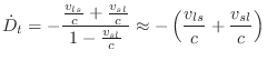
That is, the delay growth-rate,
Simulating source motion is also possible, but the relation
between delay change and desired frequency shift is more complex, viz.,
from Eq.![]() (5.2) and Eq.
(5.2) and Eq.![]() (5.6),
(5.6),
The time-varying delay line was described in §5.1. As discussed there, to implement a continuously varying delay, we add a ``delay growth parameter'' g to the delayline function in Fig.5.1, and change the line
rptr += 1; // pointer updateto
rptr += 1 - g; // pointer updateWhen g is 0, we have a fixed delay line, corresponding to
Note that when the read- and write-pointers are driven directly from a model of physical propagation-path geometry, they are always separated by predictable minimum and maximum delay intervals. This implies it is unnecessary to worry about the read-pointer passing the write-pointers or vice versa. In generic frequency shifters [275], or in a Doppler simulator not driven by a changing geometry, a pointer cross-fade scheme may be necessary when the read- and write-pointers get too close to each other.
Multiple Read Pointers
Using multiple read pointers, multiple listeners can be simulated. Furthermore, each read-pointer signal can be filtered to simulate propagation losses and radiation characteristics of the source in the direction of the listener. The read-pointers can move independently to simulate the different Doppler shifts associated with different listener motions and relative source directions.
Multiple Write Pointers
It is interesting to consider also what effects can be achieved using multiple interpolating write pointers. From the considerations in §5.7.1, we see that multiple write-pointers correspond to multiple write-heads on a magnetic tape recorder. If they are arranged at a fixed spacing, they are equivalent to multiple read pointers, providing a basic multipath simulation. If, however, the write pointers are moving independently, they induce independent Doppler shifts due to source motion. In particular, each write-pointer can lay down a signal from a separate source to a single listener with its own Doppler shift. Furthermore, each write-signal can be passed through its own filter. Such an individualized source filter can implement all filtering incurred along the propagation path from each source to the listener.
When all write pointers have the same input signal, their filters can be implemented using a series chain in which the outputs of successive filters in the chain correspond to progressively longer propagation paths (progressively more filtering). Such an implementation can greatly reduce the filter order required for propagation paths longer than the shortest.
The write-pointers may cross each other with no ill effects, since all but the first6.8 simply sum into the shared delay line.
We have seen that a single delay line can be used to simulate any
number of moving listeners (§5.7.3) or any number of moving
sources. However, when simulating both multiple listeners and
multiple sources, it is not possible to share a single delay line.
This is because the different listeners do not see the same Doppler
shift for each moving source, and while the listener's read-pointer
motion can be adjusted to correct for the Doppler shift seen from any
particular source, it cannot correct for more than one in general.
Thus, in general, we need as many delay lines as there are sources or
listeners, whichever is smaller. More precisely, if there are ![]() moving sources and
moving sources and ![]() moving listeners, simulation requires
moving listeners, simulation requires
![]() delay lines.
delay lines.
Stereo Processing
As a special case, stereo processing of any number of sources can be accomplished using two delay lines, corresponding to left and right stereo channels. The stereo mix may contain a panned mixture of any number sources, each with its own stereo placement, path filtering, and Doppler shift. The two stereo outputs may correspond to ``left and right ears,'' or, more generally, to left- and right-channel microphones in a studio recording set-up.
System Block Diagram
A schematic diagram of a stereo multiple-source simulation is shown in Fig.5.6. To simplify the layout, the input and output signals are all on the right in the diagram. For further simplicity, only one input source is shown. Additional input sources are handled identically, summing into the same delay lines in the same way.
![\includegraphics[width=0.8\twidth]{eps/bdiag}](http://www.dsprelated.com/josimages_new/pasp/img1284.png) |
The input source signal first passes through filter ![]() , which
provides time-invariant filtering common to all propagation
paths. The left- and right-channel filters
, which
provides time-invariant filtering common to all propagation
paths. The left- and right-channel filters
![]() and
and
![]() are typically low-order, linear, time-varying
filters implementing the time-varying characteristics of the shortest
(time-varying) propagation path from the source to each listener.
(The
are typically low-order, linear, time-varying
filters implementing the time-varying characteristics of the shortest
(time-varying) propagation path from the source to each listener.
(The ![]() superscript here indicates a time-varying filter.) These
filter outputs sum into the delay lines at arbitrary
(time-varying) locations using interpolating writes.
The zero signals entering each delay line on the
left can be omitted if the left-most filter overwrites delay memory
instead of summing into it.
superscript here indicates a time-varying filter.) These
filter outputs sum into the delay lines at arbitrary
(time-varying) locations using interpolating writes.
The zero signals entering each delay line on the
left can be omitted if the left-most filter overwrites delay memory
instead of summing into it.
The outputs of
![]() and
and
![]() in Fig.5.6
correspond to the ``direct signal'' from the moving source, when a
direct signal exists. These filters may incorporate modulation of
losses due to the changing propagation distance from the moving source
to each listener, and they may include dynamic equalization
corresponding to the changing radiation strength in different
directions from the moving (and possibly turning) source toward each
listener.
in Fig.5.6
correspond to the ``direct signal'' from the moving source, when a
direct signal exists. These filters may incorporate modulation of
losses due to the changing propagation distance from the moving source
to each listener, and they may include dynamic equalization
corresponding to the changing radiation strength in different
directions from the moving (and possibly turning) source toward each
listener.
The next trio of filters in Fig.5.6, ![]() ,
,
![]() ,
and
,
and
![]() , correspond to the next-to-shortest acoustic propagation
path, typically the ``first reflection,'' such as from a wall close to
the source. Since a reflection path is longer than the direct path, and since a reflection
itself can attenuate (or scatter) an incident sound ray, there is
generally more filtering required relative to the direct signal. This
additional filtering can be decomposed into its fixed component
, correspond to the next-to-shortest acoustic propagation
path, typically the ``first reflection,'' such as from a wall close to
the source. Since a reflection path is longer than the direct path, and since a reflection
itself can attenuate (or scatter) an incident sound ray, there is
generally more filtering required relative to the direct signal. This
additional filtering can be decomposed into its fixed component
![]() and time-varying components
and time-varying components
![]() and
and
![]() .
.
Note that acceptable results may be obtained without implementing all
of the filters indicated in Fig.5.6. Furthermore, it can be
convenient to incorporate ![]() into
into
![]() and
and
![]() when doing so does not increase their orders
significantly.
when doing so does not increase their orders
significantly.
Note also that the source-filters
![]() and
and
![]() may include HRTF filtering [57,545]
in order to impart illusory angles of arrival in 3D space.
may include HRTF filtering [57,545]
in order to impart illusory angles of arrival in 3D space.
Chorus Effect
The chorus effect (or ``choralizer'') is any signal processor which makes one sound source (such as a voice) sound like many such sources singing (or playing) in unison. Since performance in unison is never exact, chorus effects simulate this by making independently modified copies of the input signal. Modifications may include
- (1)
- delay,
- (2)
- frequency shift, and
- (3)
- amplitude modulation.
The typical chorus effect today is based on several time-varying delay lines which accomplishes (1) and (2) in a qualitative fashion. Reverb generally provides (3) incidentally. Before digital delay lines, analog LC ladder networks were used as an approximation, beginning in the early 1940s in the Hammond organ [59, p. 731].
An efficient chorus-effect implementation may be based on multiple interpolating taps working on a single delay line. The taps oscillate back and forth about the positions they would have while implementing a fixed tapped delay line. The tap modulation frequency may be set to achieve a prescribed frequency-shift via the Doppler effect. Each tap should be individually spatialized; in the case of stereo, each tap can be panned to its own stereo position.
The Leslie
The Leslie, named after its inventor, Don Leslie,6.9 is a popular audio processor used with electronic organs and other instruments [59,189]. It employs a rotating horn and rotating speaker port to ``choralize'' the sound. Since the horn rotates within a cabinet, the listener hears multiple reflections at different Doppler shifts, giving a kind of chorus effect. Additionally, the Leslie amplifier distorts at high volumes, producing a pleasing ``growl'' highly prized by keyboard players. At the time of this writing, there is a nice Leslie Wikipedia page, including a stereo sound-example link under the first picture (that is best heard in headphones). Papers on computational audio models of the Leslie include [468,191].
The Leslie consists primarily of a rotating horn and a rotating speaker port inside a wooden cabinet enclosure [189].
Rotating Horn Simulation
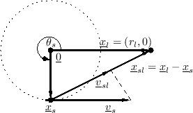
The heart of the Leslie effect is a rotating horn loudspeaker. The rotating horn from a Model 600 Leslie can be seen mounted on a microphone stand in Fig.5.7. Two horns are apparent, but one is a dummy, serving mainly to cancel the centrifugal force of the other during rotation. The Model 44W horn is identical to that of the Model 600, and evidently standard across all Leslie models [189]. For a circularly rotating horn, the source position can be approximated as
![$\displaystyle \underline{x}_s(t) = \left[\begin{array}{c} r_s\cos(\omega_m t) \\ [2pt] r_s\sin(\omega_m t) \end{array}\right] \protect$](http://www.dsprelated.com/josimages_new/pasp/img1293.png)
where
By Eq.
![\includegraphics[width=4.1in]{eps/hornrecordingr}](http://www.dsprelated.com/josimages_new/pasp/img1296.png)
![$\displaystyle \underline{v}_s(t) = \frac{d}{dt}\underline{x}_s(t) = \left[\begi...
...in(\omega_m t) \\ [2pt] r_s\omega_m\cos(\omega_m t) \end{array}\right] \protect$](http://www.dsprelated.com/josimages_new/pasp/img1297.png)
Note that the source velocity vector is always orthogonal to the source position vector, as indicated in Fig.5.8.
Since
![]() and
and
![]() are orthogonal,
the projected source velocity Eq.
are orthogonal,
the projected source velocity Eq.![]() (5.4) simplifies to
(5.4) simplifies to
Arbitrarily choosing
![$\displaystyle \underline{v}_{sl}= \frac{-r_l r_s\omega_m\sin(\omega_m t)}{r_l^2...
...l-r_s\cos(\omega_m t) \\ [2pt] -r_s\sin(\omega_m)t \end{array}\right]. \protect$](http://www.dsprelated.com/josimages_new/pasp/img1302.png)
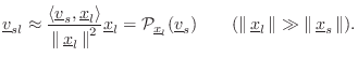
In the far field, this reduces simply to
![$\displaystyle \underline{v}_{sl}\approx -r_s\omega_m\sin(\omega_m t) \left[\begin{array}{c} 1 \\ [2pt] 0 \end{array}\right]. \protect$](http://www.dsprelated.com/josimages_new/pasp/img1303.png)
Substituting into the Doppler expression Eq.
where the approximation is valid for small Doppler shifts. Thus, in the far field, a rotating horn causes an approximately sinusoidal multiplicative frequency shift, with the amplitude given by horn length
Rotating Woofer-Port and Cabinet
It is straightforward to extend the above computational model to include the rotating woofer port (``baffle'') and wooden cabinet enclosure as follows:
- In [189], it is mentioned that an AM ``throb'' is
the main effect of the rotating woofer port. A modulated
lowpass-filter cut-off frequency has been used for this purpose by
others. Measured data can be used to construct angle-dependent
filtering in a manner analogous to that of the rotating horn, and this
``woofer filter'' runs in parallel with the rotating horn model.
- The Leslie cabinet multiply-reflects the sound emanating from
the rotating horn. The first few early reflections are simply handled
as additional sources in Fig.5.6.
- To qualitatively simulate later, more reverberant
reflections in the Leslie cabinet, we may feed a portion of the
rotating-horn and speaker-port signals to separate states of an
artificial reverberator (see Chapter 3). This reverberator
may be configured as a ``very small room'' corresponding to the
dimensions and scattering characteristics of the Leslie cabinet, and
details of the response may be calibrated using measurements of the
impulse response of the Leslie cabinet. Finally, in order to emulate
the natural spatial diversity of a radiating Leslie cabinet in a room,
``virtual cabinet vent outputs'' can be extracted from the model and
fed into separate states of a room reverberator. An alternative
time-varying FIR filtering approach based on cabinet impulse-response
measurements over a range of horn angles is described in [191].
In summary, we may use multiple interpolating write-pointers to individually simulate the early cabinet reflections, and a ``Leslie cabinet'' reverberator for handling later reflections more statistically.
Recent Research Modeling the Leslie
As mentioned above, modeling the Leslie via interpolating delay-line writes and cabinet image-sources was described in [468].6.11More recently, Leslie simulation via time-varying FIR filtering has been developed [191]. See these papers and their cited references for further details.
Next Section:
Digital Waveguide Models
Previous Section:
Delay-Line and Signal Interpolation


