


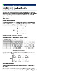
5G NR QC-LDPC Encoding Algorithm
3GPP 5G has been focused on structured LDPC codes known as quasi-cyclic low-density parity-check (QC-LDPC) codes, which exhibit advantages over other types of LDPC codes with respect to the hardware implementations of encoding and decoding using...
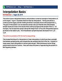
Interpolation Basics
This article covers interpolation basics, and provides a numerical example of interpolation of a time signal. Figure 1 illustrates what we mean by interpolation. The top plot shows a continuous time signal, and the middle plot shows a sampled version with sample time Ts. The goal of interpolation is to increase the sample rate such that the new (interpolated) sample values are close to the values of the continuous signal at the sample times [1]. For example, if we increase the sample rate by the integer factor of four, the interpolated signal is as shown in the bottom plot. The time between samples has been decreased from Ts to Ts/4.
Round-robin or RTOS for my embedded system
First of all, I would like to introduce myself. I am Manuel Herrera. I am starting to write blogs about the situations that I have faced over the years of my career and discussed with colleagues.To begin, I would like to open a conversation...
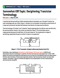
Somewhat Off Topic: Deciphering Transistor Terminology
I recently learned something mildly interesting about transistors, so I thought I'd share my new knowledge with you folks. Figure 1 shows a p-n-p transistor comprising a small block of n-type semiconductor sandwiched between two blocks of p-type...
DSP Jobs Soaring | Ready Your Interview Skills
Digital Signal Processing (DSP) technology is the cornerstone of most cutting edge technology today. For example, digital signal processing drives much of machine learning in artificial intelligence (AI). It also steers eyesight and movement...
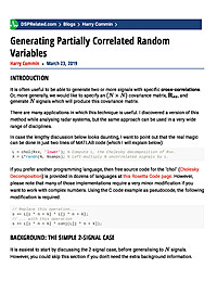
Generating Partially Correlated Random Variables
IntroductionIt is often useful to be able to generate two or more signals with specific cross-correlations. Or, more generally, we would like to specify an $\left(N \times N\right)$ covariance matrix, $\mathbf{R}_{xx}$, and generate $N$ signals...
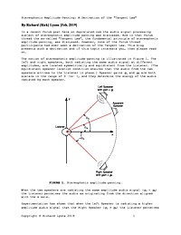
Stereophonic Amplitude-Panning: A Derivation of the "Tangent Law"
This article presents a derivation of the "Tangent Law"
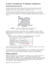
A Brief Introduction To Romberg Integration
This article briefly describes a remarkable integration algorithm, called "Romberg integration." The algorithm is used in the field of numerical analysis but it's not so well-known in the world of DSP.
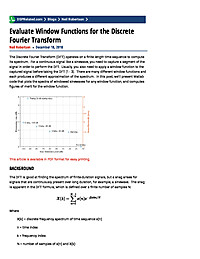
Evaluate Window Functions for the Discrete Fourier Transform
The Discrete Fourier Transform (DFT) operates on a finite length time sequence to compute its spectrum. For a continuous signal like a sinewave, you need to capture a segment of the signal in order to perform the DFT. Usually, you...
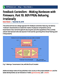
Feedback Controllers - Making Hardware with Firmware. Part 10. DSP/FPGAs Behaving Irrationally
This article will look at a design approach for feedback controllers featuring low-latency "irrational" characteristics to enable the creation of physical components such as transmission lines. Some thought will also be given as to...
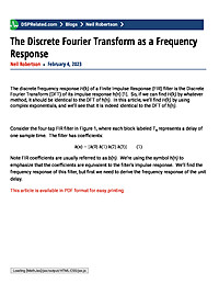
The Discrete Fourier Transform as a Frequency Response
The discrete frequency response H(k) of a Finite Impulse Response (FIR) filter is the Discrete Fourier Transform (DFT) of its impulse response h(n) [1]. So, if we can find H(k) by whatever method, it should be identical to the DFT of...
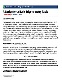
A Recipe for a Basic Trigonometry Table
Introduction This is an article that is give a better understanding to the Discrete Fourier Transform (DFT) by showing how to build a Sine and Cosine table from scratch. Along the way a recursive method is developed as a tone generator for a...
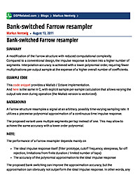
Bank-switched Farrow resampler
Bank-switched Farrow resampler Summary A modification of the Farrow structure with reduced computational complexity.Compared to a conventional design, the impulse response is broken into a higher number of segments. Interpolation accuracy is...
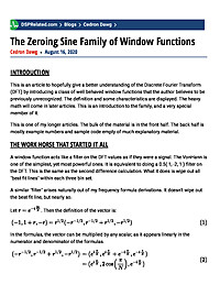
The Zeroing Sine Family of Window Functions
Introduction This is an article to hopefully give a better understanding of the Discrete Fourier Transform (DFT) by introducing a class of well behaved window functions that the author believes to be previously unrecognized. The definition...
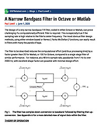
A Narrow Bandpass Filter in Octave or Matlab
The design of a very narrow bandpass FIR filter, coded in either Octave or Matlab, can prove challenging if a computationally-efficient filter is required. This is especially true if the sampling rate is high relative to the filter's center...
A Brief Introduction To Romberg Integration
This article briefly describes a remarkable integration algorithm, called "Romberg integration." The algorithm is used in the field of numerical analysis but it's not so well-known in the world of DSP.
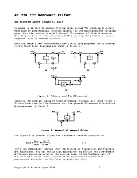
An IIR 'DC Removal' Filter
It seems to me that DC removal filters (also called "DC blocking filters") have been of some moderate interest recently on the dsprelated.com Forum web page. With that notion in mind I thought I'd post a little information, from Chapter 13 of my "Understanding DSP" book, regarding infinite impulse response (IIR) DC removal filters.
The Number 9, Not So Magic After All
This blog is not about signal processing. Rather, it discusses an interesting topic in number theory, the magic of the number 9. As such, this blog is for people who are charmed by the behavior and properties of numbers. For decades I've thought...
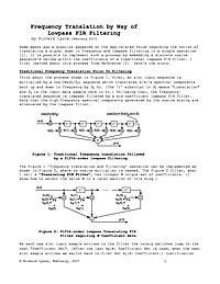
Frequency Translation by Way of Lowpass FIR Filtering
Some weeks ago a question appeared on the dsp.related Forum regarding the notion of translating a signal down in frequency and lowpass filtering in a single operation [1]. It is possible to implement such a process by embedding a discrete cosine...
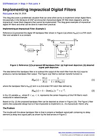
Implementing Impractical Digital Filters
This blog discusses a problematic situation that can arise when we try to implement certain digital filters. Occasionally in the literature of DSP we encounter impractical digital IIR filter block diagrams, and by impractical I mean block...


