


Example Applications of the DFT
This chapter gives a start on some applications of the DFT. First, we work through a progressive series of spectrum analysis examples using an efficient implementation of the DFT in Matlab or Octave. The various Fourier theorems provide a ``thinking vocabulary'' for understanding elements of spectral analysis. Next, the basics of linear systems theory are presented, relying heavily on the convolution theorem and properties of complex numbers. Finally, some applications of the DFT in statistical signal processing are introduced, including cross-correlation, matched filtering, system identification, power spectrum estimation, and coherence function measurement. A side topic in this chapter is practical usage of matlab for signal processing, including display of signals and spectra.
Why a DFT is usually called an FFT in practice
Practical implementations of the DFT are usually based on one of the
Cooley-Tukey ``Fast Fourier Transform'' (FFT) algorithms
[16].8.1 For
this reason, the matlab DFT function is called `fft', and the
actual algorithm used depends primarily on the transform length
![]() .8.2 The fastest FFT algorithms
generally occur when
.8.2 The fastest FFT algorithms
generally occur when ![]() is a power of 2. In practical audio signal
processing, we routinely zero-pad our FFT input buffers to the next
power of 2 in length (thereby interpolating our spectra somewhat) in
order to enjoy the power-of-2 speed advantage. Finer spectral
sampling is a typically welcome side benefit of increasing
is a power of 2. In practical audio signal
processing, we routinely zero-pad our FFT input buffers to the next
power of 2 in length (thereby interpolating our spectra somewhat) in
order to enjoy the power-of-2 speed advantage. Finer spectral
sampling is a typically welcome side benefit of increasing ![]() to the
next power of 2. Appendix A provides a short overview of some of the
better known FFT algorithms, and some pointers to literature and
online resources.
to the
next power of 2. Appendix A provides a short overview of some of the
better known FFT algorithms, and some pointers to literature and
online resources.
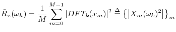
Spectrum Analysis of a Sinusoid:
Windowing, Zero-Padding, and FFT
The examples below give a progression from the most simplistic analysis up to a proper practical treatment. Careful study of these examples will teach you a lot about how spectrum analysis is carried out on real data, and provide opportunities to see the Fourier theorems in action.
FFT of a Simple Sinusoid
Our first example is an FFT of the simple sinusoid
% Example 1: FFT of a DFT-sinusoid

% Parameters:
N = 64;              % Must be a power of two
T = 1;               % Set sampling rate to 1
A = 1;               % Sinusoidal amplitude
phi = 0;             % Sinusoidal phase
f = 0.25;            % Frequency (cycles/sample)
n = [0:N-1];         % Discrete time axis
x = A*cos(2*pi*n*f*T+phi); % Sampled sinusoid
X = fft(x);          % Spectrum

% Plot time data:
figure(1);
subplot(3,1,1);
plot(n,x,'*k');
ni = [0:.1:N-1];     % Interpolated time axis
hold on;
plot(ni,A*cos(2*pi*ni*f*T+phi),'-k'); grid off;
title('Sinusoid at 1/4 the Sampling Rate');
xlabel('Time (samples)');
ylabel('Amplitude');
text(-8,1,'a)');
hold off;

% Plot spectral magnitude:
magX = abs(X);
fn = [0:1/N:1-1/N];  % Normalized frequency axis
subplot(3,1,2);
stem(fn,magX,'ok'); grid on;
xlabel('Normalized Frequency (cycles per sample))');
ylabel('Magnitude (Linear)');
text(-.11,40,'b)');

% Same thing on a dB scale:
spec = 20*log10(magX); % Spectral magnitude in dB
subplot(3,1,3);
plot(fn,spec,'--ok'); grid on;
axis([0 1 -350 50]);
xlabel('Normalized Frequency (cycles per sample))');
ylabel('Magnitude (dB)');
text(-.11,50,'c)');
cmd = ['print -deps ', '../eps/example1.eps'];
disp(cmd); eval(cmd);
![\includegraphics[width=\twidth]{eps/example1}](http://www.dsprelated.com/josimages_new/mdft/img1494.png) |
The results are shown in Fig.8.1. The time-domain signal is
shown in the upper plot (Fig.8.1a), both in pseudo-continuous
and sampled form. In the middle plot (Fig.8.1b), we see two
peaks in the magnitude spectrum, each at magnitude ![]() on a linear
scale, located at normalized frequencies
on a linear
scale, located at normalized frequencies ![]() and
and
![]() . A spectral peak amplitude of
. A spectral peak amplitude of
![]() is what we
expect, since
is what we
expect, since
The spectrum should be exactly zero at the other bin numbers. How
accurately this happens can be seen by looking on a dB scale, as shown in
Fig.8.1c. We see that the spectral magnitude in the other bins is
on the order of ![]() dB lower, which is close enough to zero for audio
work
dB lower, which is close enough to zero for audio
work
![]() .
.
FFT of a Not-So-Simple Sinusoid
Now let's increase the frequency in the above example by one-half of a bin:
% Example 2 = Example 1 with frequency between bins

f = 0.25 + 0.5/N;   % Move frequency up 1/2 bin

x = cos(2*pi*n*f*T); % Signal to analyze
X = fft(x);          % Spectrum
...                  % See Example 1 for plots and such
![\includegraphics[width=\twidth]{eps/example2}](http://www.dsprelated.com/josimages_new/mdft/img1510.png) |
The resulting magnitude spectrum is shown in Fig.8.2b and c. At this frequency, we get extensive ``spectral leakage'' into all the bins. To get an idea of where this is coming from, let's look at the periodic extension (§7.1.2) of the time waveform:
% Plot the periodic extension of the time-domain signal
plot([x,x],'--ok');
title('Time Waveform Repeated Once');
xlabel('Time (samples)'); ylabel('Amplitude');
The result is shown in Fig.8.3. Note the ``glitch'' in the middle where the signal begins its forced repetition.
![\includegraphics[width=\twidth,height=2in]{eps/waveform2}](http://www.dsprelated.com/josimages_new/mdft/img1511.png) |
FFT of a Zero-Padded Sinusoid
Looking back at Fig.8.2c, we see there are no negative dB values. Could this be right? Could the spectral magnitude at all frequencies be 1 or greater? The answer is no. To better see the true spectrum, let's use zero padding in the time domain (§7.2.7) to give ideal interpolation (§7.4.12) in the frequency domain:
zpf = 8;            % zero-padding factor
x = [cos(2*pi*n*f*T),zeros(1,(zpf-1)*N)]; % zero-padded
X = fft(x);         % interpolated spectrum
magX = abs(X);      % magnitude spectrum
...                 % waveform plot as before
nfft = zpf*N;       % FFT size = new frequency grid size
fni = [0:1.0/nfft:1-1.0/nfft]; % normalized freq axis
subplot(3,1,2);
% with interpolation, we can use solid lines '-':
plot(fni,magX,'-k'); grid on;
...
spec = 20*log10(magX); % spectral magnitude in dB
% clip below at -40 dB:
spec = max(spec,-40*ones(1,length(spec)));
...                 % plot as before
![\includegraphics[width=\twidth]{eps/example3}](http://www.dsprelated.com/josimages_new/mdft/img1512.png) |
Figure 8.4 shows the zero-padded data (top) and corresponding
interpolated spectrum on linear and dB scales (middle and bottom,
respectively). We now see that the spectrum has a regular
sidelobe structure. On the dB scale in Fig.8.4c,
negative values are now visible. In fact, it was desirable to
clip them at ![]() dB to prevent deep nulls from dominating the
display by pushing the negative vertical axis limit to
dB to prevent deep nulls from dominating the
display by pushing the negative vertical axis limit to ![]() dB or
more, as in Fig.8.1c (page
dB or
more, as in Fig.8.1c (page ![]() ). This
example shows the importance of using zero padding to interpolate
spectral displays so that the untrained eye will ``fill in'' properly
between the spectral samples.
). This
example shows the importance of using zero padding to interpolate
spectral displays so that the untrained eye will ``fill in'' properly
between the spectral samples.
Use of a Blackman Window
As Fig.8.4a suggests, the previous example can be interpreted
as using a rectangular window to select a finite segment (of
length ![]() ) from a sampled sinusoid that continues for all time.
In practical spectrum analysis, such excerpts are normally
analyzed using a window that is tapered more gracefully to
zero on the left and right. In this section, we will look at using a
Blackman window [70]8.3on our example sinusoid. The Blackman window has good (though
suboptimal) characteristics for audio work.
) from a sampled sinusoid that continues for all time.
In practical spectrum analysis, such excerpts are normally
analyzed using a window that is tapered more gracefully to
zero on the left and right. In this section, we will look at using a
Blackman window [70]8.3on our example sinusoid. The Blackman window has good (though
suboptimal) characteristics for audio work.
In Octave8.4or the Matlab Signal Processing Toolbox,8.5a Blackman window of length ![]() can be designed very easily:
can be designed very easily:
M = 64;
w = blackman(M);
Many other standard windows are defined as well, including hamming, hanning, and bartlett windows.
In Matlab without the Signal Processing Toolbox, the Blackman window is readily computed from its mathematical definition:
w = .42 - .5*cos(2*pi*(0:M-1)/(M-1)) ...
       + .08*cos(4*pi*(0:M-1)/(M-1));
Figure 8.5 shows the Blackman window and its magnitude spectrum on a dB scale. Fig.8.5c uses the more ``physical'' frequency axis in which the upper half of the FFT bin numbers are interpreted as negative frequencies. Here is the complete Matlab script for Fig.8.5:
M = 64;
w = blackman(M);
figure(1);
subplot(3,1,1); plot(w,'*'); title('Blackman Window');
xlabel('Time (samples)'); ylabel('Amplitude'); text(-8,1,'a)');

% Also show the window transform:
zpf = 8;                      % zero-padding factor
xw = [w',zeros(1,(zpf-1)*M)]; % zero-padded window
Xw = fft(xw);                 % Blackman window transform
spec = 20*log10(abs(Xw));     % Spectral magnitude in dB
spec = spec - max(spec);      % Normalize to 0 db max
nfft = zpf*M;
spec = max(spec,-100*ones(1,nfft)); % clip to -100 dB
fni = [0:1.0/nfft:1-1.0/nfft];   % Normalized frequency axis
subplot(3,1,2); plot(fni,spec,'-'); axis([0,1,-100,10]);
xlabel('Normalized Frequency (cycles per sample))');
ylabel('Magnitude (dB)'); grid; text(-.12,20,'b)');

% Replot interpreting upper bin numbers as frequencies<0:
nh = nfft/2;
specnf = [spec(nh+1:nfft),spec(1:nh)];  % see fftshift()
fninf = fni - 0.5;
subplot(3,1,3);
plot(fninf,specnf,'-'); axis([-0.5,0.5,-100,10]); grid;
xlabel('Normalized Frequency (cycles per sample))');
ylabel('Magnitude (dB)');
text(-.62,20,'c)');
cmd = ['print -deps ', '../eps/blackman.eps'];
disp(cmd); eval(cmd);
disp 'pausing for RETURN (check the plot). . .'; pause
![\includegraphics[width=\twidth]{eps/blackman}](http://www.dsprelated.com/josimages_new/mdft/img1515.png) |
Applying the Blackman Window
Now let's apply the Blackman window to the sampled sinusoid and look at the effect on the spectrum analysis:
% Windowed, zero-padded data:
n = [0:M-1];          % discrete time axis
f = 0.25 + 0.5/M;     % frequency
xw = [w .* cos(2*pi*n*f),zeros(1,(zpf-1)*M)];

% Smoothed, interpolated spectrum:
X = fft(xw);

% Plot time data:
subplot(2,1,1);
plot(xw);
title('Windowed, Zero-Padded, Sampled Sinusoid');
xlabel('Time (samples)');
ylabel('Amplitude');
text(-50,1,'a)');

% Plot spectral magnitude:
spec = 10*log10(conj(X).*X);  % Spectral magnitude in dB
spec = max(spec,-60*ones(1,nfft)); % clip to -60 dB
subplot(2,1,2);
plot(fninf,fftshift(spec),'-');
axis([-0.5,0.5,-60,40]);
title('Smoothed, Interpolated, Spectral Magnitude (dB)');
xlabel('Normalized Frequency (cycles per sample))');
ylabel('Magnitude (dB)'); grid;
text(-.6,40,'b)');
Figure 8.6 plots the zero-padded, Blackman-windowed sinusoid, along with its magnitude spectrum on a dB scale. Note that the first sidelobe (near
![\includegraphics[width=\twidth]{eps/xw}](http://www.dsprelated.com/josimages_new/mdft/img1517.png)
Hann-Windowed Complex Sinusoid
In this example, we'll perform spectrum analysis on a complex sinusoid having only a single positive frequency. We'll use the Hann window (also known as the Hanning window) which does not have as much sidelobe suppression as the Blackman window, but its main lobe is narrower. Its sidelobes ``roll off'' very quickly versus frequency. Compare with the Blackman window results to see if you can see these differences.
The Matlab script for synthesizing and plotting the Hann-windowed sinusoid is given below:
% Analysis parameters:
M = 31;         % Window length
N = 64;         % FFT length (zero padding factor near 2)

% Signal parameters:
wxT = 2*pi/4;   % Sinusoid frequency (rad/sample)
A = 1;          % Sinusoid amplitude
phix = 0;       % Sinusoid phase

% Compute the signal x:
n = [0:N-1];    % time indices for sinusoid and FFT
x = A * exp(j*wxT*n+phix); % complex sine [1,j,-1,-j...]

% Compute Hann window:
nm = [0:M-1];   % time indices for window computation
% Hann window = "raised cosine", normalization (1/M)
% chosen to give spectral peak magnitude at 1/2:
w = (1/M) * (cos((pi/M)*(nm-(M-1)/2))).^2;

wzp = [w,zeros(1,N-M)]; % zero-pad out to the length of x
xw = x .* wzp;          % apply the window w to signal x

figure(1);
subplot(1,1,1);

% Display real part of windowed signal and Hann window
plot(n,wzp,'-k'); hold on; plot(n,real(xw),'*k'); hold off;
title(['Hann Window and Windowed, Zero-Padded, ',...
       'Sinusoid (Real Part)']);
xlabel('Time (samples)'); ylabel('Amplitude');
The resulting plot of the Hann window and its use on sinusoidal data are shown in Fig.8.7.
![\includegraphics[width=\twidth]{eps/hanning}](http://www.dsprelated.com/josimages_new/mdft/img1518.png) |
Hann Window Spectrum Analysis Results
Finally, the Matlab for computing the DFT of the Hann-windowed complex sinusoid and plotting the results is listed below. To help see the full spectrum, we also compute a heavily interpolated spectrum (via zero padding as before) which we'll draw using solid lines.
% Compute the spectrum and its alternative forms:
Xw = fft(xw);              % FFT of windowed data
fn = [0:1.0/N:1-1.0/N];    % Normalized frequency axis
spec = 20*log10(abs(Xw));  % Spectral magnitude in dB
% Since the nulls can go to minus infinity, clip at -100 dB:
spec = max(spec,-100*ones(1,length(spec)));
phs = angle(Xw);           % Spectral phase in radians
phsu = unwrap(phs);        % Unwrapped spectral phase

% Compute heavily interpolated versions for comparison:
Nzp = 16;                   % Zero-padding factor
Nfft = N*Nzp;               % Increased FFT size
xwi = [xw,zeros(1,Nfft-N)]; % New zero-padded FFT buffer
Xwi = fft(xwi);             % Compute interpolated spectrum
fni = [0:1.0/Nfft:1.0-1.0/Nfft]; % Normalized freq axis
speci = 20*log10(abs(Xwi)); % Interpolated spec mag (dB)
speci = max(speci,-100*ones(1,length(speci))); % clip
phsi = angle(Xwi);          % Interpolated phase
phsiu = unwrap(phsi);       % Unwrapped interpolated phase

figure(1);
subplot(2,1,1);

plot(fn,abs(Xw),'*k'); hold on;
plot(fni,abs(Xwi),'-k'); hold off;
title('Spectral Magnitude');
xlabel('Normalized Frequency (cycles per sample))');
ylabel('Amplitude (linear)');

subplot(2,1,2);

% Same thing on a dB scale
plot(fn,spec,'*k'); hold on; plot(fni,speci,'-k'); hold off;
title('Spectral Magnitude (dB)');
xlabel('Normalized Frequency (cycles per sample))');
ylabel('Magnitude (dB)');

cmd = ['print -deps ', 'specmag.eps']; disp(cmd); eval(cmd);
disp 'pausing for RETURN (check the plot). . .'; pause

figure(1);
subplot(2,1,1);
plot(fn,phs,'*k'); hold on; plot(fni,phsi,'-k'); hold off;
title('Spectral Phase');
xlabel('Normalized Frequency (cycles per sample))');
ylabel('Phase (rad)'); grid;
subplot(2,1,2);
plot(fn,phsu,'*k'); hold on; plot(fni,phsiu,'-k'); hold off;
title('Unwrapped Spectral Phase');
xlabel('Normalized Frequency (cycles per sample))');
ylabel('Phase (rad)'); grid;
cmd = ['print -deps ', 'specphs.eps']; disp(cmd); eval(cmd);
Figure 8.8 shows the spectral magnitude and Fig.8.9 the spectral phase.
![\includegraphics[width=\twidth]{eps/specmag}](http://www.dsprelated.com/josimages_new/mdft/img1519.png)
There are no negative-frequency components in Fig.8.8 because
we are analyzing a complex sinusoid
![]() ,
which has frequency
,
which has frequency ![]() only, with no component at
only, with no component at ![]() .
.
Notice how difficult it would be to correctly interpret the shape of the ``sidelobes'' without zero padding. The asterisks correspond to a zero-padding factor of 2, already twice as much as needed to preserve all spectral information faithfully, but not enough to clearly outline the sidelobes in a spectral magnitude plot.
Spectral Phase
As for the phase of the spectrum, what do we expect? We have chosen
the sinusoid phase offset to be zero. The window is causal and
symmetric about its middle. Therefore, we expect a linear phase term
with slope
![]() samples (as discussed in connection with the
shift theorem in §7.4.4).
Also, the window transform has sidelobes which cause a phase of
samples (as discussed in connection with the
shift theorem in §7.4.4).
Also, the window transform has sidelobes which cause a phase of ![]() radians to switch in and out. Thus, we expect to see samples of a
straight line (with slope
radians to switch in and out. Thus, we expect to see samples of a
straight line (with slope ![]() samples) across the main lobe of the
window transform, together with a switching offset by
samples) across the main lobe of the
window transform, together with a switching offset by ![]() in every
other sidelobe away from the main lobe, starting with the immediately
adjacent sidelobes.
in every
other sidelobe away from the main lobe, starting with the immediately
adjacent sidelobes.
In Fig.8.9(a), we can see the negatively sloped line
across the main lobe of the window transform, but the sidelobes are
hard to follow. Even the unwrapped phase in Fig.8.9(b)
is not as clear as it could be. This is because a phase jump of ![]() radians and
radians and ![]() radians are equally valid, as is any odd multiple
of
radians are equally valid, as is any odd multiple
of ![]() radians. In the case of the unwrapped phase, all phase jumps
are by
radians. In the case of the unwrapped phase, all phase jumps
are by ![]() starting near frequency
starting near frequency ![]() .
Figure 8.9(c) shows what could be
considered the ``canonical'' unwrapped phase for this example: We see
a linear phase segment across the main lobe as before, and outside the
main lobe, we have a continuation of that linear phase across all of
the positive sidelobes, and only a
.
Figure 8.9(c) shows what could be
considered the ``canonical'' unwrapped phase for this example: We see
a linear phase segment across the main lobe as before, and outside the
main lobe, we have a continuation of that linear phase across all of
the positive sidelobes, and only a ![]() -radian deviation from that
linear phase across the negative sidelobes. In other words, we see a
straight linear phase at the desired slope interrupted by temporary
jumps of
-radian deviation from that
linear phase across the negative sidelobes. In other words, we see a
straight linear phase at the desired slope interrupted by temporary
jumps of ![]() radians. To obtain unwrapped phase of this type, the
unwrap function needs to alternate the sign of successive
phase-jumps by
radians. To obtain unwrapped phase of this type, the
unwrap function needs to alternate the sign of successive
phase-jumps by ![]() radians; this could be implemented, for example,
by detecting jumps-by-
radians; this could be implemented, for example,
by detecting jumps-by-![]() to within some numerical tolerance and
using a bit of state to enforce alternation of
to within some numerical tolerance and
using a bit of state to enforce alternation of ![]() with
with ![]() .
.
To convert the expected phase slope from ![]() ``radians per
(rad/sec)'' to ``radians per cycle-per-sample,'' we need to multiply
by ``radians per cycle,'' or
``radians per
(rad/sec)'' to ``radians per cycle-per-sample,'' we need to multiply
by ``radians per cycle,'' or ![]() . Thus, in
Fig.8.9(c), we expect a slope of
. Thus, in
Fig.8.9(c), we expect a slope of ![]() radians
per unit normalized frequency, or
radians
per unit normalized frequency, or ![]() radians per
radians per ![]() cycles-per-sample, and this looks about right, judging from the plot.
cycles-per-sample, and this looks about right, judging from the plot.

Raw spectral phase and its interpolation 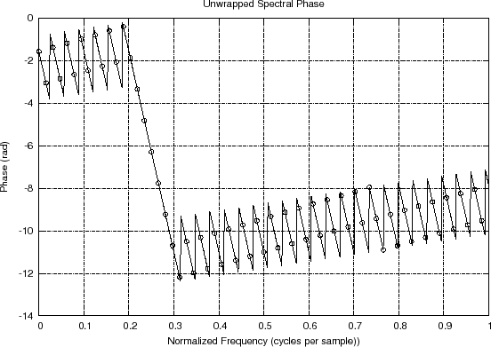
Unwrapped spectral phase and its interpolation 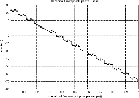
Canonically unwrapped spectral phase and its interpolation |
Spectrograms
The spectrogram is a basic tool in audio spectral analysis and other fields. It has been applied extensively in speech analysis [18,64]. The spectrogram can be defined as an intensity plot (usually on a log scale, such as dB) of the Short-Time Fourier Transform (STFT) magnitude. The STFT is simply a sequence of FFTs of windowed data segments, where the windows are usually allowed to overlap in time, typically by 25-50% [3,70]. It is an important representation of audio data because human hearing is based on a kind of real-time spectrogram encoded by the cochlea of the inner ear [49]. The spectrogram has been used extensively in the field of computer music as a guide during the development of sound synthesis algorithms. When working with an appropriate synthesis model, matching the spectrogram often corresponds to matching the sound extremely well. In fact, spectral modeling synthesis (SMS) is based on synthesizing the short-time spectrum directly by some means [86].
Spectrogram of Speech
![\includegraphics[width=\twidth]{eps/speechspgm}](http://www.dsprelated.com/josimages_new/mdft/img1531.png)
An example spectrogram for recorded speech data is shown in Fig.8.10. It was generated using the Matlab code displayed in Fig.8.11. The function spectrogram is listed in §I.5. The spectrogram is computed as a sequence of FFTs of windowed data segments. The spectrogram is plotted by spectrogram using imagesc.
[y,fs,bits] = wavread('SpeechSample.wav');
soundsc(y,fs); % Let's hear it
% for classic look:
colormap('gray'); map = colormap; imap = flipud(map);
M = round(0.02*fs);  % 20 ms window is typical
N = 2^nextpow2(4*M); % zero padding for interpolation
w = 0.54 - 0.46 * cos(2*pi*[0:M-1]/(M-1)); % w = hamming(M);
colormap(imap); % Octave wants it here
spectrogram(y,N,fs,w,-M/8,1,60);
colormap(imap); % Matlab wants it here
title('Hi - This is <you-know-who> ');
ylim([0,(fs/2)/1000]); % don't plot neg. frequencies
|
In this example, the Hamming window length was chosen to be 20 ms, as is typical in speech analysis. This is short enough so that any single 20 ms frame will typically contain data from only one phoneme,8.6 yet long enough that it will include at least two periods of the fundamental frequency during voiced speech, assuming the lowest voiced pitch to be around 100 Hz.
More generally, for speech and the singing voice (and any periodic tone), the STFT analysis parameters are chosen to trade off among the following conflicting criteria:
- The harmonics should be resolved.
- Pitch and formant variations should be closely followed.
Filters and Convolution
A reason for the importance of convolution (defined in §7.2.4) is that every linear time-invariant system8.7can be represented by a convolution. Thus, in the convolution equation
we may interpret
![\includegraphics[scale=0.8]{eps/filterbox}](http://www.dsprelated.com/josimages_new/mdft/img1533.png)
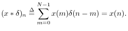
The impulse or ``unit pulse'' signal is defined by
![$\displaystyle \delta(n) \isdef \left\{\begin{array}{ll}
1, & n=0 \\ [5pt]
0, & n\neq 0. \\
\end{array} \right.
$](http://www.dsprelated.com/josimages_new/mdft/img1534.png)
The impulse signal is the identity element under convolution, since
It turns out in general that every linear time-invariant (LTI) system
(filter) is completely described by its impulse response [68].
No matter
what the LTI system is, we can feed it an impulse, record what comes
out, call it ![]() , and implement the system by convolving the input
signal
, and implement the system by convolving the input
signal ![]() with the impulse response
with the impulse response ![]() . In other words, every LTI
system has a
convolution representation in terms of its impulse response.
. In other words, every LTI
system has a
convolution representation in terms of its impulse response.
Frequency Response
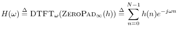
Definition: The frequency response of an LTI filter may be defined
as the Fourier transform of its impulse response. In particular, for
finite, discrete-time signals
![]() , the sampled frequency
response may be defined as
, the sampled frequency
response may be defined as
Amplitude Response
Definition: The amplitude response of a filter is defined as
the magnitude of the frequency response
Phase Response
Definition: The phase response of a filter is defined as
the phase of its frequency response:
The topics touched upon in this section are developed more fully in the next book [68] in the music signal processing series mentioned in the preface.
Correlation Analysis
The correlation operator (defined in §7.2.5) plays a major role in statistical signal processing. For a proper development, see, e.g., [27,33,65]. This section introduces only some of the most basic elements of statistical signal processing in a simplified manner, with emphasis on illustrating applications of the DFT.
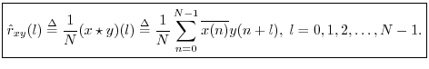
Cross-Correlation
Definition: The circular cross-correlation of two signals ![]() and
and
![]() in
in ![]() may be defined by
may be defined by
The term ``cross-correlation'' comes from
statistics, and what we have defined here is more properly
called a ``sample cross-correlation.''
That is,
![]() is an
estimator8.8 of the true
cross-correlation
is an
estimator8.8 of the true
cross-correlation ![]() which is an assumed statistical property
of the signal itself. This definition of a sample cross-correlation is only valid for
stationary stochastic processes, e.g., ``steady noises'' that
sound unchanged over time. The statistics of a stationary stochastic
process are by definition time invariant, thereby allowing
time-averages to be used for estimating statistics such
as cross-correlations. For brevity below, we will typically
not include ``sample'' qualifier, because all computational
methods discussed will be sample-based methods intended for use on
stationary data segments.
which is an assumed statistical property
of the signal itself. This definition of a sample cross-correlation is only valid for
stationary stochastic processes, e.g., ``steady noises'' that
sound unchanged over time. The statistics of a stationary stochastic
process are by definition time invariant, thereby allowing
time-averages to be used for estimating statistics such
as cross-correlations. For brevity below, we will typically
not include ``sample'' qualifier, because all computational
methods discussed will be sample-based methods intended for use on
stationary data segments.
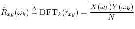
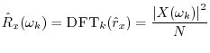
The DFT of the cross-correlation may be called the cross-spectral density, or ``cross-power spectrum,'' or even simply ``cross-spectrum'':
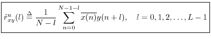
Unbiased Cross-Correlation
Recall that the cross-correlation operator is cyclic (circular)
since ![]() is interpreted modulo
is interpreted modulo ![]() . In practice, we are normally
interested in estimating the acyclic cross-correlation
between two signals. For this (more realistic) case, we may define
instead the unbiased cross-correlation
. In practice, we are normally
interested in estimating the acyclic cross-correlation
between two signals. For this (more realistic) case, we may define
instead the unbiased cross-correlation
An unbiased acyclic cross-correlation may be computed faster via DFT (FFT) methods using zero padding:
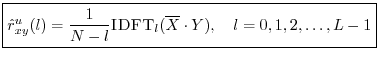
![\begin{eqnarray*}
X &=& \hbox{\sc DFT}[\hbox{\sc CausalZeroPad}_{N+L-1}(x)]\\
Y &=& \hbox{\sc DFT}[\hbox{\sc CausalZeroPad}_{N+L-1}(y)].
\end{eqnarray*}](http://www.dsprelated.com/josimages_new/mdft/img1562.png)
Note that ![]() and
and ![]() belong to
belong to ![]() while
while ![]() and
and ![]() belong to
belong to
![]() . The zero-padding may be causal (as defined in
§7.2.8)
because the signals are assumed to be be stationary, in which case all
signal statistics are time-invariant. As usual when embedding acyclic
correlation (or convolution) within the cyclic variant given by the
DFT, sufficient zero-padding is provided so that only zeros are ``time
aliased'' (wrapped around in time) by modulo indexing.
. The zero-padding may be causal (as defined in
§7.2.8)
because the signals are assumed to be be stationary, in which case all
signal statistics are time-invariant. As usual when embedding acyclic
correlation (or convolution) within the cyclic variant given by the
DFT, sufficient zero-padding is provided so that only zeros are ``time
aliased'' (wrapped around in time) by modulo indexing.
Cross-correlation is used extensively in audio signal processing for applications such as time scale modification, pitch shifting, click removal, and many others.
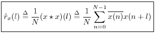
Autocorrelation
The cross-correlation of a signal with itself gives its autocorrelation:
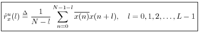
The unbiased cross-correlation similarly reduces to an unbiased
autocorrelation when ![]() :
:
The DFT of the true autocorrelation function
![]() is the (sampled)
power spectral density (PSD), or power spectrum, and may
be denoted
is the (sampled)
power spectral density (PSD), or power spectrum, and may
be denoted
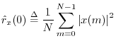
At lag zero, the autocorrelation function reduces to the average power (mean square) which we defined in §5.8:
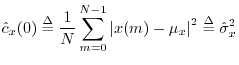
Replacing ``correlation'' with ``covariance'' in the above definitions gives corresponding zero-mean versions. For example, we may define the sample circular cross-covariance as
![$\displaystyle \zbox {{\hat c}_{xy}(n)
\isdef \frac{1}{N}\sum_{m=0}^{N-1}\overline{[x(m)-\mu_x]} [y(m+n)-\mu_y].}
$](http://www.dsprelated.com/josimages_new/mdft/img1575.png)
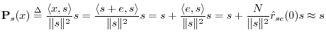
Matched Filtering
The cross-correlation function is used extensively in pattern
recognition and signal detection. We know from Chapter 5
that projecting one signal onto another is a means of measuring how
much of the second signal is present in the first. This can be used
to ``detect'' the presence of known signals as components of more
complicated signals. As a simple example, suppose we record ![]() which we think consists of a signal
which we think consists of a signal ![]() that we are looking for
plus some additive measurement noise
that we are looking for
plus some additive measurement noise ![]() . That is, we assume the
signal model
. That is, we assume the
signal model
![]() . Then the projection of
. Then the projection of ![]() onto
onto ![]() is
(recalling §5.9.9)
is
(recalling §5.9.9)
In the same way that FFT convolution is faster than direct convolution (see Table 7.1), cross-correlation and matched filtering are generally carried out most efficiently using an FFT algorithm (Appendix A).
FIR System Identification
Estimating an impulse response from input-output measurements is called system identification, and a large literature exists on this topic (e.g., [39]).
Cross-correlation can be used to compute the impulse response ![]() of a filter from the cross-correlation of its input and output signals
of a filter from the cross-correlation of its input and output signals
![]() and
and
![]() , respectively. To see this, note that, by
the correlation theorem,
, respectively. To see this, note that, by
the correlation theorem,

% sidex.m - Demonstration of the use of FFT cross- % correlation to compute the impulse response % of a filter given its input and output. % This is called "FIR system identification". Nx = 32; % input signal length Nh = 10; % filter length Ny = Nx+Nh-1; % max output signal length % FFT size to accommodate cross-correlation: Nfft = 2^nextpow2(Ny); % FFT wants power of 2 x = rand(1,Nx); % input signal = noise %x = 1:Nx; % input signal = ramp h = [1:Nh]; % the filter xzp = [x,zeros(1,Nfft-Nx)]; % zero-padded input yzp = filter(h,1,xzp); % apply the filter X = fft(xzp); % input spectrum Y = fft(yzp); % output spectrum Rxx = conj(X) .* X; % energy spectrum of x Rxy = conj(X) .* Y; % cross-energy spectrum Hxy = Rxy ./ Rxx; % should be the freq. response hxy = ifft(Hxy); % should be the imp. response hxy(1:Nh) % print estimated impulse response freqz(hxy,1,Nfft); % plot estimated freq response err = norm(hxy - [h,zeros(1,Nfft-Nh)])/norm(h); disp(sprintf(['Impulse Response Error = ',... '%0.14f%%'],100*err)); err = norm(Hxy-fft([h,zeros(1,Nfft-Nh)]))/norm(h); disp(sprintf(['Frequency Response Error = ',... '%0.14f%%'],100*err)); |
Power Spectral Density Estimation
Welch's method [85] (or the periodogram method
[20]) for estimating power spectral densities (PSD) is carried
out by dividing the time signal into successive blocks, and
averaging squared-magnitude DFTs of the signal blocks. Let
![]() ,
,
![]() , denote the
, denote the ![]() th block of the
signal
th block of the
signal
![]() , with
, with ![]() denoting the number of blocks.
Then the Welch PSD estimate is given by
denoting the number of blocks.
Then the Welch PSD estimate is given by
where ``
Recall that
![]() which is
circular (cyclic) autocorrelation. To obtain an acyclic
autocorrelation instead, we may use zero padding in the time
domain, as described in §8.4.2.
That is, we can replace
which is
circular (cyclic) autocorrelation. To obtain an acyclic
autocorrelation instead, we may use zero padding in the time
domain, as described in §8.4.2.
That is, we can replace ![]() above by
above by
![]() .8.12Although this fixes the ``wrap-around problem'', the estimator is
still biased because its expected value is the true
autocorrelation
.8.12Although this fixes the ``wrap-around problem'', the estimator is
still biased because its expected value is the true
autocorrelation ![]() weighted by
weighted by ![]() . This bias is equivalent
to multiplying the correlation in the ``lag domain'' by a
triangular window (also called a ``Bartlett window''). The bias
can be removed by simply dividing it out, as in Eq.
. This bias is equivalent
to multiplying the correlation in the ``lag domain'' by a
triangular window (also called a ``Bartlett window''). The bias
can be removed by simply dividing it out, as in Eq.![]() (8.2), but it is
common to retain the Bartlett weighting since it merely corresponds to
smoothing the power spectrum (or cross-spectrum) with a
sinc
(8.2), but it is
common to retain the Bartlett weighting since it merely corresponds to
smoothing the power spectrum (or cross-spectrum) with a
sinc![]() kernel;8.13it also down-weights the less reliable large-lag
estimates, weighting each lag by the number of lagged products that
were summed.
kernel;8.13it also down-weights the less reliable large-lag
estimates, weighting each lag by the number of lagged products that
were summed.
Since
![]() , and since the DFT
is a linear operator (§7.4.1), averaging
magnitude-squared DFTs
, and since the DFT
is a linear operator (§7.4.1), averaging
magnitude-squared DFTs
![]() is equivalent, in
principle, to estimating block autocorrelations
is equivalent, in
principle, to estimating block autocorrelations
![]() , averaging
them, and taking a DFT of the average. However, this would normally
be slower.
, averaging
them, and taking a DFT of the average. However, this would normally
be slower.
We return to power spectral density estimation in Book IV [70] of the music signal processing series.
Coherence Function
A function related to cross-correlation is the coherence function, defined in terms of power spectral densities and the cross-spectral density by
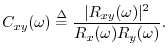

The coherence
![]() is a real function between zero and one
which gives a measure of correlation between
is a real function between zero and one
which gives a measure of correlation between ![]() and
and ![]() at
each frequency
at
each frequency ![]() . For example, imagine that
. For example, imagine that ![]() is produced
from
is produced
from ![]() via an LTI filtering operation:
via an LTI filtering operation:
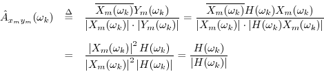
so that the coherence function becomes

A common use for the coherence function is in the validation of
input/output data collected in an acoustics experiment for purposes of
system identification. For example, ![]() might be a known
signal which is input to an unknown system, such as a reverberant
room, say, and
might be a known
signal which is input to an unknown system, such as a reverberant
room, say, and ![]() is the recorded response of the room. Ideally,
the coherence should be
is the recorded response of the room. Ideally,
the coherence should be ![]() at all frequencies. However, if the
microphone is situated at a null in the room response for some
frequency, it may record mostly noise at that frequency. This is
indicated in the measured coherence by a significant dip below 1. An
example is shown in Book III [69] for the case of a measured
guitar-bridge admittance.
A more elementary example is given in the next section.
at all frequencies. However, if the
microphone is situated at a null in the room response for some
frequency, it may record mostly noise at that frequency. This is
indicated in the measured coherence by a significant dip below 1. An
example is shown in Book III [69] for the case of a measured
guitar-bridge admittance.
A more elementary example is given in the next section.
Coherence Function in Matlab
In Matlab and Octave, cohere(x,y,M) computes the coherence
function ![]() using successive DFTs of length
using successive DFTs of length ![]() with a Hanning
window and 50% overlap. (The window and overlap can be controlled
via additional optional arguments.) The matlab listing in
Fig.8.14 illustrates cohere on a simple example.
Figure 8.15 shows a plot of cxyM for this example.
We see a coherence peak at frequency
with a Hanning
window and 50% overlap. (The window and overlap can be controlled
via additional optional arguments.) The matlab listing in
Fig.8.14 illustrates cohere on a simple example.
Figure 8.15 shows a plot of cxyM for this example.
We see a coherence peak at frequency ![]() cycles/sample, as
expected, but there are also two rather large coherence samples on
either side of the main peak. These are expected as well, since the
true cross-spectrum for this case is a critically sampled Hanning
window transform. (A window transform is critically sampled whenever
the window length equals the DFT length.)
cycles/sample, as
expected, but there are also two rather large coherence samples on
either side of the main peak. These are expected as well, since the
true cross-spectrum for this case is a critically sampled Hanning
window transform. (A window transform is critically sampled whenever
the window length equals the DFT length.)
% Illustrate estimation of coherence function 'cohere' % in the Matlab Signal Processing Toolbox % or Octave with Octave Forge: N = 1024; % number of samples x=randn(1,N); % Gaussian noise y=randn(1,N); % Uncorrelated noise f0 = 1/4; % Frequency of high coherence nT = [0:N-1]; % Time axis w0 = 2*pi*f0; x = x + cos(w0*nT); % Let something be correlated p = 2*pi*rand(1,1); % Phase is irrelevant y = y + cos(w0*nT+p); M = round(sqrt(N)); % Typical window length [cxyM,w] = cohere(x,y,M); % Do the work figure(1); clf; stem(w/2,cxyM,'*'); % w goes from 0 to 1 (odd convention) legend(''); % needed in Octave grid on; ylabel('Coherence'); xlabel('Normalized Frequency (cycles/sample)'); axis([0 1/2 0 1]); replot; % Needed in Octave saveplot('../eps/coherex.eps'); % compatibility utility |
![\includegraphics[width=\twidth]{eps/coherex}](http://www.dsprelated.com/josimages_new/mdft/img1617.png)
Note that more than one frame must be averaged to obtain a coherence
less than one. For example, changing the cohere call in the
above example to
``cxyN = cohere(x,y,N);''
produces all ones in cxyN, because no averaging is
performed.
Recommended Further Reading
We are now finished developing the mathematics of the DFT and a first look at some of its applications. The sequel consists of appendices which fill in more elementary background and supplement the prior development with related new topics, such as the Fourier transform and FFT algorithm.
For further study, one may, of course, continue on to Book II (Introduction to Digital Filter Theory [68]) in the music signal processing series (mentioned in the preface). Alternatively and in addition, the references cited in the bibliography can provide further guidance.
Next Section:
Fast Fourier Transform (FFT) Algorithms
Previous Section:
Fourier Theorems for the DFT


