


More General Finite-Difference Methods
The FDA and bilinear transform of the previous sections can be viewed
as first-order conformal maps from the analog ![]() plane to the digital
plane to the digital
![]() plane. These maps are one-to-one and therefore non-aliasing. The
FDA performs well at low frequencies relative to the sampling rate,
but it introduces artificial damping at high frequencies. The
bilinear transform preserves the frequency axis exactly, but over a
warped frequency scale. Being first order, both maps preserve the
number of poles and zeros in the model.
plane. These maps are one-to-one and therefore non-aliasing. The
FDA performs well at low frequencies relative to the sampling rate,
but it introduces artificial damping at high frequencies. The
bilinear transform preserves the frequency axis exactly, but over a
warped frequency scale. Being first order, both maps preserve the
number of poles and zeros in the model.
We may only think in terms of mapping the ![]() plane to the
plane to the ![]() plane
for linear, time-invariant systems. This is because Laplace
transform analysis is not defined for nonlinear and/or time-varying
differential equations (no
plane
for linear, time-invariant systems. This is because Laplace
transform analysis is not defined for nonlinear and/or time-varying
differential equations (no ![]() plane). Therefore, such systems are
instead digitized by some form of numerical integration to
produce solutions that are ideally sampled versions of the
continuous-time solutions. It is often necessary to work at sampling
rates much higher than the desired audio sampling rate, due to the
bandwidth-expanding effects of nonlinear elements in the
continuous-time system.
plane). Therefore, such systems are
instead digitized by some form of numerical integration to
produce solutions that are ideally sampled versions of the
continuous-time solutions. It is often necessary to work at sampling
rates much higher than the desired audio sampling rate, due to the
bandwidth-expanding effects of nonlinear elements in the
continuous-time system.
A tutorial review of numerical solutions of Ordinary Differential Equations (ODE), including nonlinear systems, with examples in the realm of audio effects (such as a diode clipper), is given in [555]. Finite difference schemes specifically designed for nonlinear discrete-time simulation, such as the energy-preserving ``Kirchoff-Carrier nonlinear string model'' and ``von Karman nonlinear plate model'', are discussed in [53].
The remaining sections here summarize a few of the more elementary techniques discussed in [555].
General Nonlinear ODE
In state-space form (§1.3.7) [449],8.7a general class of ![]() th-order Ordinary Differential Equations (ODE),
can be written as
th-order Ordinary Differential Equations (ODE),
can be written as
where
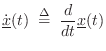
In the linear, time-invariant (LTI) case, Eq.![]() (7.8) can be
expressed in the usual state-space form for LTI continuous-time
systems:
(7.8) can be
expressed in the usual state-space form for LTI continuous-time
systems:
In this case, standard methods for converting a filter from continuous to discrete time may be used, such as the FDA (§7.3.1) and bilinear transform (§7.3.2).8.8
Forward Euler Method
The finite-difference approximation (Eq.![]() (7.2)) with the
derivative evaluated at time
(7.2)) with the
derivative evaluated at time ![]() yields the forward Euler
method of numerical integration:
yields the forward Euler
method of numerical integration:
where
Because each iteration of the forward Euler method depends only on
past quantities, it is termed an explicit method. In the LTI
case, an explicit method corresponds to a causal digital filter
[449]. Methods that depend on current and/or future
solution samples (i.e.,
![]() for
for ![]() ) are
called implicit methods. When a nonlinear
numerical-integration method is implicit, each step forward in time
typically uses some number of iterations of Newton's Method (see
§7.4.5 below).
) are
called implicit methods. When a nonlinear
numerical-integration method is implicit, each step forward in time
typically uses some number of iterations of Newton's Method (see
§7.4.5 below).
Backward Euler Method
An example of an implicit method is the backward Euler method:
Because the derivative is now evaluated at time
Trapezoidal Rule
The trapezoidal rule is defined by
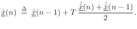
Thus, the trapezoidal rule is driven by the average of the derivative estimates at times
The trapezoidal rule gets its name from the fact that it approximates
an integral by summing the areas of trapezoids. This can be seen by writing
Eq.![]() (7.12) as
(7.12) as
An interesting fact about the trapezoidal rule is that it is
equivalent to the bilinear transform in the linear,
time-invariant case. Carrying Eq.![]() (7.12) to the frequency domain
gives
(7.12) to the frequency domain
gives
![\begin{eqnarray*}
X(z) &=& z^{-1}X(z) + T\, \frac{s X(z) + z^{-1}s X(z)]}{2}\\
...
...gleftrightarrow\quad s &=& \frac{2}{T}\frac{1-z^{-1}}{1+z^{-1}}.
\end{eqnarray*}](http://www.dsprelated.com/josimages_new/pasp/img1709.png)
Newton's Method of Nonlinear Minimization
Newton's method [162],[166, p. 143] finds the minimum of a nonlinear (scalar) function of several variables by locally approximating the function by a quadratic surface, and then stepping to the bottom of that ``bowl'', which generally requires a matrix inversion. Newton's method therefore requires the function to be ``close to quadratic'', and its effectiveness is directly tied to the accuracy of that assumption. For smooth functions, Newton's method gives very rapid quadratic convergence in the last stages of iteration. Quadratic convergence implies, for example, that the number of significant digits in the minimizer approximately doubles each iteration.
Newton's method may be derived as follows: Suppose we wish to minimize
the real, positive function
![]() with respect to
with respect to
![]() . The
vector Taylor expansion [546] of
. The
vector Taylor expansion [546] of
![]() about
about
![]() gives
gives
Applying Eq.
where
When the
![]() is any quadratic form in
is any quadratic form in
![]() , then
, then
![]() , and
Newton's method produces
, and
Newton's method produces
![]() in one iteration; that is,
in one iteration; that is,
![]() for every
for every
![]() .
.
Semi-Implicit Methods
A semi-implicit method for numerical integration is based on an
implicit method by using only one iteration of Newton's method
[354,555]. This effectively converts the implicit
method into a corresponding explicit method. Best results are
obtained for highly oversampled systems (i.e., ![]() is larger
than typical audio sampling rates).
is larger
than typical audio sampling rates).
Semi-Implicit Backward Euler
The semi-implicit backward Euler method is defined by [555]
![$\displaystyle \underline{\hat{x}}(n) \isdefs \underline{\hat{x}}(n-1) + T\, \frac{f[n,\underline{\hat{x}}(n-1)]}{1-T\,\ddot{\underline{\hat{x}}}(n-1)} \protect$](http://www.dsprelated.com/josimages_new/pasp/img1725.png)
where
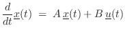
Semi-Implicit Trapezoidal Rule
The semi-implicit trapezoidal rule method is given by [555]
![$\displaystyle \underline{\hat{x}}(n) \isdefs \underline{\hat{x}}(n-1) + \frac{T...
...rline{\hat{x}}(n-1)]}{1-\frac{T}{2}\,\ddot{\underline{\hat{x}}}(n-1)}. \protect$](http://www.dsprelated.com/josimages_new/pasp/img1728.png)
Summary
We have looked at a number of methods for solving nonlinear ordinary differential equations, including explicit, implicit, and semi-implicit numerical integration methods. Specific methods included the explicit forward Euler (similar to the finite difference approximation of §7.3.1), backward Euler (implicit), trapezoidal rule (implicit, and equivalent to the bilinear transform of §7.3.2 in the LTI case), and semi-implicit variants of the backward Euler and trapezoidal methods.
As demonstrated and discussed further in [555], implicit methods are generally more accurate than explicit methods for nonlinear systems, with semi-implicit methods (§7.4.6) typically falling somewhere in between. Semi-implicit methods therefore provide a source of improved explicit methods. See [555] and the references therein for a discussion of accuracy and stability of such schemes, as well as applied examples.
Further Reading in Nonlinear Methods
Other well known numerical integration methods for ODEs include second-order backward difference formulas (commonly used in circuit simulation [555]), the fourth-order Runge-Kutta method [99], and their various explicit, implicit, and semi-implicit variations. See [555] for further discussion of these and related finite-difference schemes, and for application examples in the virtual analog area (digitization of musically useful analog circuits). Specific digitization problems addressed in [555] include electric-guitar distortion devices [553,556], the classic ``tone stack'' [552] (an often-used bass, midrange, and treble control circuit in guitar amplifiers), the Moog VCF, and other electronic components of amplifiers and effects. Also discussed in [555] is the ``K Method'' for nonlinear system digitization, with comparison to nonlinear wave digital filters (see Appendix F for an introduction to linear wave digital filters).
The topic of real-time finite difference schemes for virtual analog systems remains a lively research topic [554,338,293,84,264,364,397].
For Partial Differential Equations (PDEs), in which spatial derivatives are mixed with time derivatives, the finite-difference approach remains fundamental. An introduction and summary for the LTI case appear in Appendix D. See [53] for a detailed development of finite difference schemes for solving PDEs, both linear and nonlinear, applied to digital sound synthesis. Physical systems considered in [53] include bars, stiff strings, bow coupling, hammers and mallets, coupled strings and bars, nonlinear strings and plates, and acoustic tubes (voice, wind instruments). In addition to numerous finite-difference schemes, there are chapters on finite-element methods and spectral methods.
Next Section:
Summary of Lumped Modeling
Previous Section:
Digitization of Lumped Models


