


Finite-Difference Schemes
This appendix gives some simplified definitions and results from the subject of finite-difference schemes for numerically solving partial differential equations. Excellent references on this subject include Bilbao [53,55] and Strikwerda [481].
The simplifications adopted here are that we will exclude nonlinear and time-varying partial differential equations (PDEs). We will furthermore assume constant step-sizes (sampling intervals) when converting PDEs to finite-difference schemes (FDSs), i.e., sampling rates along time and space will be constant. Accordingly, we will assume that all initial conditions are bandlimited to less than half the spatial sampling rate, and that all excitations over time (such as summing input signals or ``moving boundary conditions'') will be bandlimited to less than half the temporal sampling rate. In short, the simplifications adopted here make the subject of partial differential equations isomorphic to that of linear systems theory [449]. For a more general and traditional treatment of PDEs and their associated finite-difference schemes, see, e.g., [481].
Finite-Difference Schemes
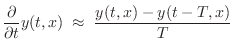
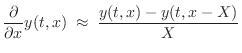
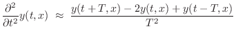
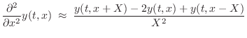
Finite-Difference Schemes (FDSs) aim to solve differential
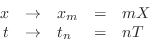
equations by means of finite differences. For example, as discussed
in §C.2, if ![]() denotes the displacement in meters of a vibrating
string at time
denotes the displacement in meters of a vibrating
string at time ![]() seconds and position
seconds and position ![]() meters, we may approximate
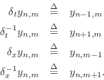
the first- and second-order partial derivatives by
meters, we may approximate
the first- and second-order partial derivatives by
where
where
The FDS is called explicit because it was possible to solve for the state at time
Convergence
A finite-difference scheme is said to be convergent if all of its solutions in response to initial conditions and excitations converge pointwise to the corresponding solutions of the original differential equation as the step size(s) approach zero.
In other words, as the step-size(s) shrink, the FDS solution must improve, ultimately converging to the corresponding solution of the original differential equation at every point of the domain.
In the vibrating string example, the limit is taken as the step sizes
(sampling intervals) ![]() and
and ![]() approach zero. Since the
finite-difference approximations in
Eq.
approach zero. Since the
finite-difference approximations in
Eq.![]() (D.1) converge in the limit to the very definitions of the
corresponding partial derivatives, we expect the FDS in Eq.
(D.1) converge in the limit to the very definitions of the
corresponding partial derivatives, we expect the FDS in Eq.![]() (D.3)
based on these approximations to be convergent (and it is).
(D.3)
based on these approximations to be convergent (and it is).
In establishing convergence, it is necessary to provide that any initial conditions and boundary conditions in the finite-difference scheme converge to those of the continuous differential equation, in the limit. See [481] for a more detailed discussion of this topic.
The Lax-Richtmyer equivalence theorem provides a means of showing convergence of a finite-difference scheme by showing it is both consistent and stable (and that the initial-value problem is well posed) [481]. The following subsections give basic definitions for these terms which applicable to our simplified scenario (linear, shift-invariant, fixed sampling rates).
Consistency
A finite-difference scheme is said to be
consistent with the original
partial differential equation if, given any sufficiently
differentiable function ![]() , the differential equation operating
on
, the differential equation operating
on ![]() approaches the value of the finite difference equation
operating on
approaches the value of the finite difference equation
operating on ![]() , as
, as ![]() and
and ![]() approach zero.
approach zero.
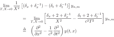
Thus, in the ideal string example, to show the consistency of Eq.![]() (D.3)
we must show that
(D.3)
we must show that
![$\displaystyle \left(\frac{\partial^2}{\partial x^2}
- \frac{1}{c^2}
\frac{\par...
...eft[
(\delta_x + \delta_x^{-1})
-
(\delta_t + \delta_t^{-1})
\right] y_{n,m}
$](http://www.dsprelated.com/josimages_new/pasp/img4454.png)
In particular, we have
In taking the limit as ![]() and
and ![]() approach zero, we must maintain
the relationship
approach zero, we must maintain
the relationship ![]() , and we must scale the FDS by
, and we must scale the FDS by ![]() in
order to achieve an exact result:
in
order to achieve an exact result:
as required. Thus, the FDS is consistent. See, e.g., [481] for more examples.
In summary, consistency of a finite-difference scheme means that, in the limit as the sampling intervals approach zero, the original PDE is obtained from the FDS.
Well Posed Initial-Value Problem
For a proper authoritative definition of ``well posed'' in the field of finite-difference schemes, see, e.g., [481]. The definition we will use here is less general in that it excludes amplitude growth from initial conditions which is faster than polynomial in time.
We will say that an initial-value problem is well posed if the linear system defined by the PDE, together with any bounded initial conditions is marginally stable.
As discussed in [449], a system is defined to be stable when its response to bounded initial conditions approaches zero as time goes to infinity. If the response fails to approach zero but does not exponentially grow over time (the lossless case), it is called marginally stable.
In the literature on finite-difference schemes, lossless systems are classified as stable [481]. However, in this book series, lossless systems are not considered stable, but only marginally stable.
When marginally stable systems are allowed, it is necessary to accommodate polynomial growth with respect to time. As is well known in linear systems theory, repeated poles can yield polynomial growth [449]. A very simple example is the ordinary differential equation (ODE)
When all poles of the system are strictly in the left-half of the
Laplace-transform ![]() plane, the system is stable, even when
the poles are repeated. This is because exponentials are faster than
polynomials, so that any amount of exponential decay will eventually
overtake polynomial growth and drag it to zero in the limit.
plane, the system is stable, even when
the poles are repeated. This is because exponentials are faster than
polynomials, so that any amount of exponential decay will eventually
overtake polynomial growth and drag it to zero in the limit.
Marginally stable systems arise often in computational physical
modeling. In particular, the ideal string is only marginally stable,
since it is lossless. Even a simple unaccelerated mass, sliding on a
frictionless surface, is described by a marginally stable PDE when the
position of the mass is used as a state variable (see
§7.1.2). Given any nonzero initial velocity, the position
of the mass approaches either ![]() or
or ![]() infinity, exactly as in the
infinity, exactly as in the
![]() example above. To avoid unbounded growth in practical
systems, it is often preferable to avoid the use of displacement as a
state variable. For ideal strings and freely sliding masses, force
and velocity are usually good choices.
example above. To avoid unbounded growth in practical
systems, it is often preferable to avoid the use of displacement as a
state variable. For ideal strings and freely sliding masses, force
and velocity are usually good choices.
It should perhaps be emphasized that the term ``well posed'' normally allows for more general energy growth at a rate which can be bounded over all initial conditions [481]. In this book, however, the ``marginally stable'' case (at most polynomial growth) is what we need. The reason is simply that we wish to excluded unstable PDEs as a modeling target. Note, however, that unstable systems can be used profitable over carefully limited time durations (see §9.7.2 for an example).
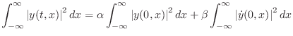
In the ideal vibrating string, energy is conserved. Therefore, it is a
marginally stable system. To show mathematically that the PDE
Eq.![]() (D.2) is marginally stable, we may show that
(D.2) is marginally stable, we may show that
Note that solutions on the ideal string are not bounded, since, for
example, an infinitely long string (non-terminated) can be initialized
with a constant positive velocity everywhere along its length. This
corresponds physically to a nonzero transverse momentum, which is
conserved. Therefore, the string will depart in the positive ![]() direction, with an average displacement that grows linearly with
direction, with an average displacement that grows linearly with ![]() .
.
The well-posedness of a class of damped PDEs used in string modeling is analyzed in §D.2.2.
A Class of Well Posed Damped PDEs
A large class of well posed PDEs is given by [45]
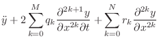
Thus, to the ideal string wave equation Eq.
To show Eq.![]() (D.5) is well posed [45], we must
show that the roots of the characteristic polynomial equation
(§D.3) have negative real parts, i.e., that they correspond to
decaying exponentials instead of growing exponentials. To do this, we
may insert the general eigensolution
(D.5) is well posed [45], we must
show that the roots of the characteristic polynomial equation
(§D.3) have negative real parts, i.e., that they correspond to
decaying exponentials instead of growing exponentials. To do this, we
may insert the general eigensolution
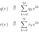
Let's now set ![]() , where
, where
![]() is radian spatial
frequency (called the ``wavenumber'' in acoustics) and of course
is radian spatial
frequency (called the ``wavenumber'' in acoustics) and of course
![]() , thereby converting the implicit spatial Laplace
transform to a spatial Fourier transform. Since there are only even
powers of the spatial Laplace transform variable
, thereby converting the implicit spatial Laplace
transform to a spatial Fourier transform. Since there are only even
powers of the spatial Laplace transform variable ![]() , the polynomials
, the polynomials
![]() and
and ![]() are real. Therefore, the roots of the
characteristic polynomial equation (the natural frequencies of the
time response of the system), are given by
are real. Therefore, the roots of the
characteristic polynomial equation (the natural frequencies of the
time response of the system), are given by
Proof that the Third-Order Time Derivative is Ill Posed
For its tutorial value, let's also show that the PDE of Ruiz
[392] is ill posed, i.e., that at least one component of the
solution is a growing exponential. In this case, setting
![]() in Eq.
in Eq.![]() (C.28), which we restate as
(C.28), which we restate as
It is interesting to note that Ruiz discovered the exponentially growing solution, but simply dropped it as being non-physical. In the work of Chaigne and Askenfelt [77], it is believed that the finite difference approximation itself provided the damping necessary to eliminate the unstable solution [45]. (See §7.3.2 for a discussion of how finite difference approximations can introduce damping.) Since the damping effect is sampling-rate dependent, there is an upper bound to the sampling rate that can be used before an unstable mode appears.
Stability of a Finite-Difference Scheme
A finite-difference scheme is said to be stable if it forms a digital filter which is at least marginally stable [449].
To distinguish between the stable and marginally stable cases, we may classify a finite-difference scheme as strictly stable, marginally stable, or unstable.
Lax-Richtmyer equivalence theorem
The Lax-Richtmyer equivalence theorem states that ``a consistent finite-difference scheme for a partial differential equation for which the initial-value problem is well posed is convergent if and only if it is stable.'' For a proof, see [481, Ch. 10].
Passivity of a Finite-Difference Scheme
A condition stronger than stability as defined above is passivity. Passivity is not a traditional metric for finite-difference scheme analysis, but it arises naturally in special cases such as wave digital filters (§F.1) and digital waveguide networks [55,35]. In such modeling frameworks, all signals have a physical interpretation as wave variables, and therefore a physical energy can be associated with them. Moreover, each delay element can be associated with some real wave impedance. In such situations, passivity can be defined as the case in which all impedances are nonnegative. When complex, they must be positive real (see §C.11.2).
To define passivity for all linear, shift-invariant finite difference schemes, irrespective of whether or not they are based on an impedance description, we will say that a finite-difference scheme is passive if all of its internal modes are stable. Thus, passivity is sufficient, but not necessary, for stability. In other words, there are finite difference schemes which are stable but not passive [55]. A stable FDS can have internal unstable modes which are not excited by initial conditions, or which always cancel out in pairs. A passive FDS cannot have such ``hidden'' unstable modes.
The absence of hidden modes can be ascertained by converting the FDS to a state-space model and checking that it is controllable (from initial conditions and/or excitations) and observable [449]. When the initial conditions can set the entire initial state of the FDS, it is then controllable from initial conditions, and only observability needs to be checked. A simple example of an unobservable mode is the second harmonic of an ideal string (and all even-numbered harmonics) when the only output observation is the midpoint of the string.
Summary
In summary, we have defined the following terms from the analysis of finite-difference schemes for the linear shift-invariant case with constant sampling rates:
- PDE well posed
 PDE at least marginally stable
- FDS consistent
FDS shift operator
 PDE operator as
- FDS stable
stable or marginally stable as a digital filter
- FDS strictly stable
stable as a digital filter
- FDS marginally stable
marginally stable as a digital filter
Convergence in Audio Applications
Because the range of human hearing is bounded (nominally between 20 and 20 kHz), spectral components of a signal outside this range are not audible. Therefore, when the solution to a differential equation is to be considered an audio signal, there are frequency regions over which convergence is not a requirement.
Instead of pointwise convergence, we may ask for the following two properties:
- Superposition holds.
- Convergence occurs within the frequency band of human hearing.
In many cases, such as in digital waveguide modeling of vibrating strings, we can do better than convergence. We can construct finite difference schemes which agree with the corresponding continuous solutions exactly at the sample points. (See §C.4.1.)
Characteristic Polynomial Equation
The characteristic polynomial equation for a linear PDE with
constant coefficients is obtained by taking the 2D Laplace transform
of the PDE with respect to ![]() and
and ![]() . A simple way of doing this is
to substitute the general eigensolution
. A simple way of doing this is
to substitute the general eigensolution
into the PDE, where
As a simple example, the ideal-string wave equation (analyzed in §C.1) is a simple second-order PDE given by
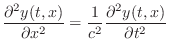
where
Substituting Eq.![]() (D.6) into Eq.
(D.6) into Eq.![]() (D.7) results in the following
characteristic polynomial equation:
(D.7) results in the following
characteristic polynomial equation:
Von Neumann Analysis
Von Neumann analysis is used to verify the stability of a finite-difference scheme. We will only consider one time dimension, but any number of spatial dimensions.
The procedure, in principle, is to perform a spatial Fourier transform along all spatial dimensions, thereby reducing the finite-difference scheme to a time recursion in terms of the spatial Fourier transform of the system. The system is then stable if this time recursion is at least marginally stable as a digital filter.
Let's apply von Neumann analysis to the finite-difference scheme for
the ideal vibrating string Eq.![]() (D.3):
(D.3):
where
A method equivalent to checking the pole radii, and typically used
when the time recursion is first order, is to compute the
amplification factor as the complex gain ![]() in
the relation
in
the relation
Since the finite-difference scheme of the ideal vibrating string is so
simple, let's find the two poles. Taking the z transform of Eq.![]() (D.8)
yields
(D.8)
yields
![$\displaystyle \left\vert z\right\vert^2 = c_k^2 \pm (c_k^2 - 1) =
\left\{\begi...
...eq 1 \\ [5pt]
[1,1], & \left\vert c_k\right\vert\leq 1 \\
\end{array}\right..
$](http://www.dsprelated.com/josimages_new/pasp/img4501.png)
In summary, von Neumann analysis verifies that no spatial Fourier components in the system are growing exponentially with respect to time.
Next Section:
Equivalence of Digital Waveguide and Finite Difference Schemes
Previous Section:
Digital Waveguide Theory


