


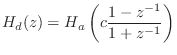
Digitization of Lumped Models
Since lumped models are described by differential equations, they are digitized (brought into the digital-signal domain) by converting them to corresponding finite-difference equations (or simply ``difference equations''). General aspects of finite difference schemes are discussed in Appendix D. This chapter introduces a couple of elementary methods in common use:
Note that digitization by the bilinear transform is closely related to the Wave Digital Filter (WDF) method introduced in Appendix F. Section 9.3.1 discusses a bilinearly transformed mass colliding with a digital waveguide string (an idealized struck-string example).
Finite Difference Approximation
A finite difference approximation (FDA) approximates derivatives with finite differences, i.e.,
![$\displaystyle \frac{d}{dt} x(t) \isdefs \lim_{\delta\to 0} \frac{x(t) - x(t-\delta)}{\delta} \;\approx\; \frac{x(n T)-x[(n-1)T]}{T} \protect$](http://www.dsprelated.com/josimages_new/pasp/img1643.png)
for sufficiently small
Equation (7.2) is also known as the backward difference approximation of differentiation.
See §C.2.1 for a discussion of using the FDA to model ideal vibrating strings.
FDA in the Frequency Domain
Viewing Eq.![]() (7.2) in the frequency domain, the ideal
differentiator transfer-function is
(7.2) in the frequency domain, the ideal
differentiator transfer-function is ![]() , which can be viewed as
the Laplace transform of the operator
, which can be viewed as
the Laplace transform of the operator ![]() (left-hand side of
Eq.
(left-hand side of
Eq.![]() (7.2)). Moving to the right-hand side, the z transform of the
first-order difference operator is
(7.2)). Moving to the right-hand side, the z transform of the
first-order difference operator is
![]() . Thus, in the
frequency domain, the finite-difference approximation may be performed
by making the substitution
. Thus, in the
frequency domain, the finite-difference approximation may be performed
by making the substitution
in any continuous-time transfer function (Laplace transform of an integro-differential operator) to obtain a discrete-time transfer function (z transform of a finite-difference operator).
The inverse of substitution Eq.![]() (7.3) is
(7.3) is
As discussed in §8.3.1, the FDA is a special case of the
matched ![]() transformation applied to the point
transformation applied to the point ![]() .
.
Note that the FDA does not alias, since the conformal mapping
![]() is one to one. However, it does warp the poles and zeros in a
way which may not be desirable, as discussed further on p.
is one to one. However, it does warp the poles and zeros in a
way which may not be desirable, as discussed further on p. ![]() below.
below.
Delay Operator Notation
It is convenient to think of the FDA in terms of time-domain
difference operators using a delay operator notation. The
delay operator ![]() is defined by
is defined by
The obvious definition for the second derivative is

However, a better definition is the centered finite difference
where
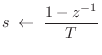
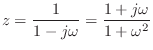
Bilinear Transformation
The bilinear transform is defined by the substitution
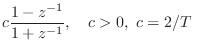 (typically)
where
It can be seen that analog dc (![]() ) maps to digital dc (
) maps to digital dc (![]() ) and
the highest analog frequency (
) and
the highest analog frequency (![]() ) maps to the highest digital
frequency (
) maps to the highest digital
frequency (![]() ). It is easy to show that the entire
). It is easy to show that the entire ![]() axis
in the
axis
in the ![]() plane (where
plane (where
![]() ) is mapped exactly
once around the unit circle in the
) is mapped exactly
once around the unit circle in the ![]() plane (rather than
summing around it infinitely many times, or ``aliasing'' as it does in
ordinary sampling). With
plane (rather than
summing around it infinitely many times, or ``aliasing'' as it does in
ordinary sampling). With ![]() real and positive, the left-half
real and positive, the left-half ![]() plane maps to the interior of the unit circle, and the right-half
plane maps to the interior of the unit circle, and the right-half ![]() plane maps outside the unit circle. This means stability is
preserved when mapping a continuous-time transfer function to
discrete time.
plane maps outside the unit circle. This means stability is
preserved when mapping a continuous-time transfer function to
discrete time.
Another valuable property of the bilinear transform is that
order is preserved. That is, an ![]() th-order
th-order ![]() -plane transfer
function carries over to an
-plane transfer
function carries over to an ![]() th-order
th-order ![]() -plane transfer function.
(Order in both cases equals the maximum of the degrees of the
numerator and denominator polynomials [449]).8.6
-plane transfer function.
(Order in both cases equals the maximum of the degrees of the
numerator and denominator polynomials [449]).8.6
The constant ![]() provides one remaining degree of freedom which can be used
to map any particular finite frequency from the
provides one remaining degree of freedom which can be used
to map any particular finite frequency from the ![]() axis in the
axis in the ![]() plane to a particular desired location on the unit circle
plane to a particular desired location on the unit circle
![]() in the
in the ![]() plane. All other frequencies will be warped. In
particular, approaching half the sampling rate, the frequency axis
compresses more and more. Note that at most one resonant frequency can be
preserved under the bilinear transformation of a mass-spring-dashpot
system. On the other hand, filters having a single transition frequency,
such as lowpass or highpass filters, map beautifully under the bilinear
transform; one simply uses
plane. All other frequencies will be warped. In
particular, approaching half the sampling rate, the frequency axis
compresses more and more. Note that at most one resonant frequency can be
preserved under the bilinear transformation of a mass-spring-dashpot
system. On the other hand, filters having a single transition frequency,
such as lowpass or highpass filters, map beautifully under the bilinear
transform; one simply uses ![]() to map the cut-off frequency where it
belongs, and the response looks great. In particular, ``equal ripple'' is
preserved for optimal filters of the elliptic and Chebyshev types because
the values taken on by the frequency response are identical in both cases;
only the frequency axis is warped.
to map the cut-off frequency where it
belongs, and the response looks great. In particular, ``equal ripple'' is
preserved for optimal filters of the elliptic and Chebyshev types because
the values taken on by the frequency response are identical in both cases;
only the frequency axis is warped.
The bilinear transform is often used to design digital filters from analog prototype filters [343]. An on-line introduction is given in [449].
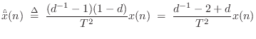
Finite Difference Approximation vs. Bilinear Transform
Recall that the Finite Difference Approximation (FDA) defines the
elementary differentiator by
![]() (ignoring the
scale factor
(ignoring the
scale factor ![]() for now), and this approximates the ideal transfer
function
for now), and this approximates the ideal transfer
function ![]() by
by
![]() . The bilinear transform
calls instead for the transfer function
. The bilinear transform
calls instead for the transfer function
![]() (again
dropping the scale factor) which introduces a pole at
(again
dropping the scale factor) which introduces a pole at ![]() and gives
us the recursion
and gives
us the recursion
![]() .
Note that this new pole is right on the unit circle and is therefore
undamped. Any signal energy at half the sampling rate will circulate
forever in the recursion, and due to round-off error, it will tend to
grow. This is therefore a potentially problematic revision of the
differentiator. To get something more practical, we need to specify
that the filter frequency response approximate
.
Note that this new pole is right on the unit circle and is therefore
undamped. Any signal energy at half the sampling rate will circulate
forever in the recursion, and due to round-off error, it will tend to
grow. This is therefore a potentially problematic revision of the
differentiator. To get something more practical, we need to specify
that the filter frequency response approximate
![]() over a
finite range of frequencies
over a
finite range of frequencies
![]() , where
, where
![]() , above which we allow the response to ``roll off''
to zero. This is how we pose the differentiator problem in terms of
general purpose filter design (see §8.6) [362].
, above which we allow the response to ``roll off''
to zero. This is how we pose the differentiator problem in terms of
general purpose filter design (see §8.6) [362].
To understand the properties of the finite difference approximation in the
frequency domain, we may look at the properties of its ![]() -plane
to
-plane
to ![]() -plane mapping
-plane mapping

Setting ![]() to 1 for simplicity and solving the FDA mapping for z gives
to 1 for simplicity and solving the FDA mapping for z gives
![\includegraphics[width=3in]{eps/lfdacirc}](http://www.dsprelated.com/josimages_new/pasp/img1678.png)
Under the FDA, analog and digital frequency axes coincide well enough at
very low frequencies (high sampling rates), but at high frequencies
relative to the sampling rate, artificial damping is introduced as
the image of the ![]() axis diverges away from the unit circle.
axis diverges away from the unit circle.
While the bilinear transform ``warps'' the frequency axis, we can say the FDA ``doubly warps'' the frequency axis: It has a progressive, compressive warping in the direction of increasing frequency, like the bilinear transform, but unlike the bilinear transform, it also warps normal to the frequency axis.
Consider a point traversing the upper half of the unit circle in the z
plane, starting at ![]() and ending at
and ending at ![]() . At dc, the FDA is
perfect, but as we proceed out along the unit circle, we diverge from the
. At dc, the FDA is
perfect, but as we proceed out along the unit circle, we diverge from the
![]() axis image and carve an arc somewhere out in the image of the
right-half
axis image and carve an arc somewhere out in the image of the
right-half ![]() plane. This has the effect of introducing an artificial
damping.
plane. This has the effect of introducing an artificial
damping.
Consider, for example, an undamped mass-spring system. There will be a
complex conjugate pair of poles on the ![]() axis in the
axis in the ![]() plane. After
the FDA, those poles will be inside the unit circle, and therefore damped
in the digital counterpart. The higher the resonance frequency, the larger
the damping. It is even possible for unstable
plane. After
the FDA, those poles will be inside the unit circle, and therefore damped
in the digital counterpart. The higher the resonance frequency, the larger
the damping. It is even possible for unstable ![]() -plane poles to be mapped
to stable
-plane poles to be mapped
to stable ![]() -plane poles.
-plane poles.
In summary, both the bilinear transform and the FDA preserve order,
stability, and positive realness. They are both free of aliasing, high
frequencies are compressively warped, and both become ideal at dc, or as
![]() approaches
approaches ![]() . However, at frequencies significantly above
zero relative to the sampling rate, only the FDA introduces artificial
damping. The bilinear transform maps the continuous-time frequency axis in
the
. However, at frequencies significantly above
zero relative to the sampling rate, only the FDA introduces artificial
damping. The bilinear transform maps the continuous-time frequency axis in
the ![]() (the
(the ![]() axis) plane precisely to the discrete-time frequency
axis in the
axis) plane precisely to the discrete-time frequency
axis in the ![]() plane (the unit circle).
plane (the unit circle).
Application of the Bilinear Transform
The impedance of a mass in the frequency domain is
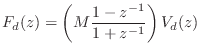
![\begin{eqnarray*}
(1+z^{-1})F_d(z) &=& M (1-z^{-1}) V_d(z) \\
\;\longleftrighta...
...
\,\,\Rightarrow\,\,f_d(n) &=& M[v_d(n) - v_d(n-1)] - f_d(n-1).
\end{eqnarray*}](http://www.dsprelated.com/josimages_new/pasp/img1686.png)
This difference equation is diagrammed in Fig. 7.16. We recognize this recursive digital filter as the direct form I structure. The direct-form II structure is obtained by commuting the feedforward and feedback portions and noting that the two delay elements contain the same value and can therefore be shared [449]. The two other major filter-section forms are obtained by transposing the two direct forms by exchanging the input and output, and reversing all arrows. (This is a special case of Mason's Gain Formula which works for the single-input, single-output case.) When a filter structure is transposed, its summers become branching nodes and vice versa. Further discussion of the four basic filter section forms can be found in [333].
![\includegraphics[width=4in]{eps/lmassFilterDF1}](http://www.dsprelated.com/josimages_new/pasp/img1687.png) |
Practical Considerations
While the digital mass simulator has the desirable properties of the bilinear transform,
it is also not perfect from a practical point of view:
(1) There is a pole at half the sampling rate (![]() ).
(2) There is a delay-free path from input to output.
).
(2) There is a delay-free path from input to output.
The first problem can easily be circumvented by introducing a loss factor ![]() ,
moving the pole from
,
moving the pole from ![]() to
to ![]() , where
, where ![]() and
and ![]() . This
is sometimes called the ``leaky integrator''.
. This
is sometimes called the ``leaky integrator''.
The second problem arises when making loops of elements (e.g., a mass-spring chain which forms a loop). Since the individual elements have no delay from input to output, a loop of elements is not computable using standard signal processing methods. The solution proposed by Alfred Fettweis is known as ``wave digital filters,'' a topic taken up in §F.1.
Limitations of Lumped Element Digitization
Model discretization by the FDA (§7.3.1) and bilinear transform (§7.3.2) methods are order preserving. As a result, they suffer from significant approximation error, especially at high frequencies relative to half the sampling rate. By allowing a larger order in the digital model, we may obtain arbitrarily accurate transfer-function models of LTI subsystems, as discussed in Chapter 8. Of course, in higher-order approximations, the state variables of the simulation no longer have a direct physical intepretation, and this can have implications, particularly when trying to extend to the nonlinear case. The benefits of a physical interpretation should not be given up lightly. For example, one may consider oversampling in place of going to higher-order element approximations.
Next Section:
More General Finite-Difference Methods
Previous Section:
One-Port Network Theory


