


Matrix Filter Representations
This appendix introduces various matrix representations for digital filters, including the important state space formulation. Additionally, elementary system identification based on a matrix description is described.
Introduction
It is illuminating to look at matrix representations of digital
filters.F.1Every linear digital filter can be expressed as a
constant matrix
![]() multiplying the input signal
multiplying the input signal
![]() (the
input vector) to produce the output signal (vector)
(the
input vector) to produce the output signal (vector)
![]() , i.e.,
, i.e.,
More generally, any finite-order linear operator can be
expressed as a matrix multiply. For example, the Discrete Fourier
Transform (DFT) can be represented by the ``DFT matrix''
![]() , where the column index
, where the column index ![]() and row index
and row index ![]() range from 0
to
range from 0
to ![]() [84, p. 111].F.2Even infinite-order linear operators are often thought of as matrices
having infinite extent. In summary, if a digital filter is
linear, it can be represented by a matrix.
[84, p. 111].F.2Even infinite-order linear operators are often thought of as matrices
having infinite extent. In summary, if a digital filter is
linear, it can be represented by a matrix.
General Causal Linear Filter Matrix
To be causal, the filter output at time
![]() cannot
depend on the input at any times
cannot
depend on the input at any times ![]() greater than
greater than ![]() . This implies
that a causal filter matrix must be lower triangular. That is,
it must have zeros above the main diagonal. Thus, a causal linear filter
matrix
. This implies
that a causal filter matrix must be lower triangular. That is,
it must have zeros above the main diagonal. Thus, a causal linear filter
matrix
![]() will have entries that satisfy
will have entries that satisfy ![]() for
for ![]() .
.
For example, the general ![]() causal, linear, digital-filter
matrix operating on three-sample sequences is
causal, linear, digital-filter
matrix operating on three-sample sequences is
![$\displaystyle \mathbf{h}= \left[\begin{array}{ccc}
h_{00} & 0 & 0\\ [2pt]
h_{10} & h_{11} & 0\\ [2pt]
h_{20} & h_{21} & h_{22}
\end{array}\right]
$](http://www.dsprelated.com/josimages_new/filters/img1962.png)
![$\displaystyle \left[\begin{array}{c} y_0 \\ [2pt] y_1 \\ [2pt] y_2\end{array}\r...
...left[\begin{array}{c} x_0 \\ [2pt] x_1 \\ [2pt] x_2\end{array}\right], \protect$](http://www.dsprelated.com/josimages_new/filters/img1963.png)
or, more explicitly,
While Eq.![]() (F.2) covers the general case of linear, causal, digital
filters operating on the space of three-sample sequences, it includes
time varying filters, in general. For example, the gain of the
``current input sample'' changes over time as
(F.2) covers the general case of linear, causal, digital
filters operating on the space of three-sample sequences, it includes
time varying filters, in general. For example, the gain of the
``current input sample'' changes over time as
![]() .
.
General LTI Filter Matrix
The general linear, time-invariant (LTI) matrix is Toeplitz.
A Toeplitz matrix is constant along all its diagonals.
For example, the general ![]() LTI matrix is given by
LTI matrix is given by
![$\displaystyle \mathbf{h}= \left[\begin{array}{ccc}
h_{0} & h_{-1} & h_{-2}\\ [2pt]
h_{1} & h_{0} & h_{-1}\\ [2pt]
h_{2} & h_{1} & h_{0}
\end{array}\right]
$](http://www.dsprelated.com/josimages_new/filters/img1971.png)
![$\displaystyle \mathbf{h}= \left[\begin{array}{ccc}
h_{0} & 0 & 0\\ [2pt]
h_{1} & h_{0} & 0\\ [2pt]
h_{2} & h_{1} & h_{0}
\end{array}\right].
$](http://www.dsprelated.com/josimages_new/filters/img1972.png)
![$\displaystyle \left[\begin{array}{c} y_0 \\ [2pt] y_1 \\ [2pt] y_2 \\ [2pt] y_3...
...{array}{c} x_0 \\ [2pt] x_1 \\ [2pt] x_2 \\ [2pt] 0\\ [2pt] 0\end{array}\right]$](http://www.dsprelated.com/josimages_new/filters/img1975.png) |
(F.3) |
We could add more rows to obtain more output samples, but the additional outputs would all be zero.
In general, if a causal FIR filter is length ![]() , then its order is
, then its order is
![]() , so to avoid ``cutting off'' the output signal prematurely, we
must append at least
, so to avoid ``cutting off'' the output signal prematurely, we
must append at least ![]() zeros to the input signal. Appending
zeros in this way is often called zero padding, and it is used
extensively in spectrum analysis [84]. As a specific example,
an order 5 causal FIR filter (length 6) requires 5 samples of
zero-padding on the input signal to avoid output truncation.
zeros to the input signal. Appending
zeros in this way is often called zero padding, and it is used
extensively in spectrum analysis [84]. As a specific example,
an order 5 causal FIR filter (length 6) requires 5 samples of
zero-padding on the input signal to avoid output truncation.
If the FIR filter is noncausal, then zero-padding is needed
before the input signal in order not to ``cut off'' the
``pre-ring'' of the filter (the response before time ![]() ).
).
To handle arbitrary-length input signals, keeping the filter length at 3 (an order 2 FIR filter), we may simply use a longer banded Toeplitz filter matrix:
![$\displaystyle \mathbf{h}= \left[\begin{array}{ccccccc}
h_0 & 0 & 0 & 0 & 0 & 0...
...& \\
\vdots & \vdots & \vdots & & \ddots & \ddots & \ddots
\end{array}\right]
$](http://www.dsprelated.com/josimages_new/filters/img1978.png)
Cyclic Convolution Matrix
An infinite Toeplitz matrix implements, in principle, acyclic
convolution (which is what we normally mean when we just say
``convolution''). In practice, the convolution of a signal ![]() and an
impulse response
and an
impulse response ![]() , in which both
, in which both ![]() and
and ![]() are more than a
hundred or so samples long, is typically implemented fastest using
FFT convolution (i.e., performing fast convolution using the
Fast Fourier Transform (FFT)
[84]F.3). However, the FFT computes
cyclic convolution unless sufficient zero padding is used
[84]. The matrix representation of cyclic (or ``circular'')
convolution is a circulant matrix, e.g.,
are more than a
hundred or so samples long, is typically implemented fastest using
FFT convolution (i.e., performing fast convolution using the
Fast Fourier Transform (FFT)
[84]F.3). However, the FFT computes
cyclic convolution unless sufficient zero padding is used
[84]. The matrix representation of cyclic (or ``circular'')
convolution is a circulant matrix, e.g.,
![$\displaystyle \mathbf{h}= \left[\begin{array}{cccccc}
h_0 & 0 & 0 & 0 & h_2 & ...
... h_2 & h_1 & h_0 & 0 \\ [2pt]
0 & 0 & 0 & h_2 & h_1 & h_0
\end{array}\right].
$](http://www.dsprelated.com/josimages_new/filters/img1979.png)
The DFT eigenstructure of circulant matrices is directly related to
the DFT convolution theorem [84]. The above ![]() circulant matrix
circulant matrix
![]() , when multiplied times a length 6 vector
, when multiplied times a length 6 vector
![]() ,
implements cyclic convolution of
,
implements cyclic convolution of
![]() with
with
![]() .
Using the DFT to perform the circular convolution can be expressed as
.
Using the DFT to perform the circular convolution can be expressed as

Premultiplying by the IDFT matrix
![]() yields
yields
Inverse Filters
Note that the filter matrix
![]() is often invertible
[58]. In that case, we can effectively run the filter
backwards:
is often invertible
[58]. In that case, we can effectively run the filter
backwards:
> h = toeplitz([1,2,0,0,0],[1,0,0,0,0])
h =
  1  0  0  0  0
  2  1  0  0  0
  0  2  1  0  0
  0  0  2  1  0
  0  0  0  2  1
> inv(h)
ans =
    1    0    0    0    0
   -2    1    0    0    0
    4   -2    1    0    0
   -8    4   -2    1    0
   16   -8    4   -2    1
The inverse of the FIR filter Another point to notice is that the inverse of a banded Toeplitz matrix is not banded (although the inverse of lower-triangular [causal] matrix remains lower triangular). This corresponds to the fact that the inverse of an FIR filter is an IIR filter.
State Space Realization
Above, we used a matrix multiply to represent convolution of the
filter input signal with the filter's impulse response. This only
works for FIR filters since an IIR filter would require an infinite
impulse-response matrix. IIR filters have an extensively used matrix
representation called state space form
(or ``state space realizations'').
They are especially convenient for representing filters with
multiple inputs and multiple outputs (MIMO filters).
An order ![]() digital filter with
digital filter with ![]() inputs and
inputs and ![]() outputs can be written
in state-space form as follows:
outputs can be written
in state-space form as follows:
where
State-space models are described further in Appendix G. Here, we will only give an illustrative example and make a few observations:
State Space Filter Realization Example
The digital filter having difference equation
![$\displaystyle \left[\begin{array}{c} x_1(n+1) \\ [2pt] x_2(n+1) \\ [2pt] x_3(n+1)\end{array}\right]$](http://www.dsprelated.com/josimages_new/filters/img2015.png)
![$\displaystyle \left[\begin{array}{ccc}
0 & 1 & 0\\ [2pt]
0 & 0 & 1\\ [2pt]
0.01...
...\right] +
\left[\begin{array}{c} 0 \\ [2pt] 0 \\ [2pt] 1\end{array}\right] u(n)$](http://www.dsprelated.com/josimages_new/filters/img2016.png)
![$\displaystyle \left[\begin{array}{ccc} 0 & 1 & 1\end{array}\right]
\left[\begin{array}{c} x_1(n) \\ [2pt] x_2(n) \\ [2pt] x_3(n)\end{array}\right]
\protect$](http://www.dsprelated.com/josimages_new/filters/img2017.png)
Thus,
This example is repeated using matlab in §G.7.8 (after we have covered transfer functions).
A general procedure for converting any difference equation to
state-space form is described in §G.7. The particular
state-space model shown in Eq.![]() (F.5) happens to be called
controller canonical form,
for reasons discussed in Appendix G.
The set of all state-space realizations of this filter is given by
exploring the set of all similarity transformations applied to
any particular realization, such as the control-canonical form in
Eq.
(F.5) happens to be called
controller canonical form,
for reasons discussed in Appendix G.
The set of all state-space realizations of this filter is given by
exploring the set of all similarity transformations applied to
any particular realization, such as the control-canonical form in
Eq.![]() (F.5). Similarity transformations are discussed in
§G.8, and in books on linear algebra [58].
(F.5). Similarity transformations are discussed in
§G.8, and in books on linear algebra [58].
Note that the state-space model replaces an ![]() th-order
difference equation by a vector first-order difference
equation. This provides elegant simplifications in the theory and
analysis of digital filters. For example, consider the case
th-order
difference equation by a vector first-order difference
equation. This provides elegant simplifications in the theory and
analysis of digital filters. For example, consider the case ![]() ,
and
,
and ![]() , so that Eq.
, so that Eq.![]() (F.4) reduces to
(F.4) reduces to
where
Time Domain Filter Estimation
System identification is the subject of identifying filter coefficients given measurements of the input and output signals [46,78]. For example, one application is amplifier modeling, in which we measure (1) the normal output of an electric guitar (provided by the pick-ups), and (2) the output of a microphone placed in front of the amplifier we wish to model. The guitar may be played in a variety of ways to create a collection of input/output data to use in identifying a model of the amplifier's ``sound.'' There are many commercial products which offer ``virtual amplifier'' presets developed partly in such a way.F.6 One can similarly model electric guitars themselves by measuring the pick signal delivered to the string (as the input) and the normal pick-up-mix output signal. A separate identification is needed for each switch and tone-control position. After identifying a sampling of models, ways can be found to interpolate among the sampled settings, thereby providing ``virtual'' tone-control knobs that respond like the real ones [101].
In the notation of the §F.1, assume we know
![]() and
and
![]() and wish to solve for the filter impulse response
and wish to solve for the filter impulse response
![]() . We now outline a simple yet
practical method for doing this, which follows readily from the
discussion of the previous section.
. We now outline a simple yet
practical method for doing this, which follows readily from the
discussion of the previous section.
Recall that convolution is commutative. In terms of the matrix representation of §F.3, this implies that the input signal and the filter can switch places to give
![$\displaystyle \underbrace{%
\left[\begin{array}{c}
y_0 \\ [2pt] y_1 \\ [2pt] y...
... h_2 \\ [2pt] h_3\\ [2pt] h_4\end{array}\right]}_{\displaystyle\underline{h}},
$](http://www.dsprelated.com/josimages_new/filters/img2031.png)
Here we have indicated the general case for a length
The Moore-Penrose pseudoinverse is easy to
derive.F.7 First multiply Eq.![]() (F.7) on the left by the
transpose of
(F.7) on the left by the
transpose of
![]() in order to obtain a ``square'' system of
equations:
in order to obtain a ``square'' system of
equations:
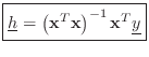
Thus,
If the input signal ![]() is an impulse
is an impulse ![]() (a 1 at time
zero and 0 at all other times), then
(a 1 at time
zero and 0 at all other times), then
![]() is simply the identity
matrix, which is its own inverse, and we obtain
is simply the identity
matrix, which is its own inverse, and we obtain
![]() . We expect
this by definition of the impulse response. More generally,
. We expect
this by definition of the impulse response. More generally,
![]() is invertible whenever the input signal is ``sufficiently
exciting'' at all frequencies. An LTI filter frequency response can
be identified only at frequencies that are excited by the input, and
the accuracy of the estimate at any given frequency can be improved by
increasing the input signal power at that frequency.
[46].
is invertible whenever the input signal is ``sufficiently
exciting'' at all frequencies. An LTI filter frequency response can
be identified only at frequencies that are excited by the input, and
the accuracy of the estimate at any given frequency can be improved by
increasing the input signal power at that frequency.
[46].
Effect of Measurement Noise
In practice, measurements are never perfect. Let
![]() denote the measured output signal, where
denote the measured output signal, where
![]() is a vector of
``measurement noise'' samples. Then we have
is a vector of
``measurement noise'' samples. Then we have
It is also straightforward to introduce a weighting function in
the least-squares estimate for
![]() by replacing
by replacing
![]() in the
derivations above by
in the
derivations above by
![]() , where
, where ![]() is any positive definite
matrix (often taken to be diagonal and positive). In the present
time-domain formulation, it is difficult to choose a
weighting function that corresponds well to audio perception.
Therefore, in audio applications, frequency-domain formulations are
generally more powerful for linear-time-invariant system
identification. A practical example is the frequency-domain
equation-error method described in §I.4.4 [78].
is any positive definite
matrix (often taken to be diagonal and positive). In the present
time-domain formulation, it is difficult to choose a
weighting function that corresponds well to audio perception.
Therefore, in audio applications, frequency-domain formulations are
generally more powerful for linear-time-invariant system
identification. A practical example is the frequency-domain
equation-error method described in §I.4.4 [78].
Matlab System Identification Example
The Octave output for the following small matlab example is listed in Fig.F.1:
delete('sid.log'); diary('sid.log'); % Log session
echo('on');       % Show commands as well as responses
N = 4;            % Input signal length
%x = rand(N,1)    % Random input signal - snapshot:
x = [0.056961, 0.081938, 0.063272, 0.672761]'
h = [1 2 3]';     % FIR filter
y = filter(h,1,x) % Filter output
xb = toeplitz(x,[x(1),zeros(1,N-1)]) % Input matrix
hhat = inv(xb' * xb) * xb' * y % Least squares estimate
% hhat = pinv(xb) * y % Numerically robust pseudoinverse
hhat2 = xb\y % Numerically superior (and faster) estimate
diary('off'); % Close log file
One fine point is the use of the syntax ``
+ echo('on');       % Show commands as well as responses
+ N = 4;            % Input signal length
+ %x = rand(N,1)    % Random input signal - snapshot:
+ x = [0.056961, 0.081938, 0.063272, 0.672761]'
x =
  0.056961
  0.081938
  0.063272
  0.672761

+ h = [1 2 3]';     % FIR filter
+ y = filter(h,1,x) % Filter output
y =
  0.056961
  0.195860
  0.398031
  1.045119

+ xb = toeplitz(x,[x(1),zeros(1,N-1)]) % Input matrix
xb =
  0.05696  0.00000  0.00000  0.00000
  0.08194  0.05696  0.00000  0.00000
  0.06327  0.08194  0.05696  0.00000
  0.67276  0.06327  0.08194  0.05696

+ hhat = inv(xb' * xb) * xb' * y % Least squares estimate
hhat =
   1.0000
   2.0000
   3.0000
   3.7060e-13

+ % hhat = pinv(xb) * y % Numerically robust pseudoinverse
+ hhat2 = xb\y % Numerically superior (and faster) estimate
hhat2 =
   1.0000
   2.0000
   3.0000
   3.6492e-16
|
Next Section:
State Space Filters
Previous Section:
Analog Filters


