


Analog Filters
For our purposes, an analog filter is any filter which operates
on continuous-time signals. In other respects, they are just
like digital filters. In particular, linear, time-invariant (LTI)
analog filters can be
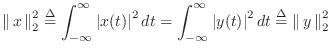
characterized by their (continuous) impulse response ![]() , where
, where ![]() is time in seconds. Instead of a difference equation, analog filters
may be described by a differential equation. Instead of using
the z transform to compute the transfer function, we use the Laplace
transform (introduced in Appendix D). Every aspect of the theory
of digital filters has its counterpart in that of analog filters. In
fact, one can think of analog filters as simply the limiting case of
digital filters as the sampling-rate is allowed to go to infinity.
is time in seconds. Instead of a difference equation, analog filters
may be described by a differential equation. Instead of using
the z transform to compute the transfer function, we use the Laplace
transform (introduced in Appendix D). Every aspect of the theory
of digital filters has its counterpart in that of analog filters. In
fact, one can think of analog filters as simply the limiting case of
digital filters as the sampling-rate is allowed to go to infinity.
In the real world, analog filters are often electrical models, or ``analogues'', of mechanical systems working in continuous time. If the physical system is LTI (e.g., consisting of elastic springs and masses which are constant over time), an LTI analog filter can be used to model it. Before the widespread use of digital computers, physical systems were simulated on so-called ``analog computers.'' An analog computer was much like an analog synthesizer providing modular building-blocks (such as ``integrators'') that could be patched together to build models of dynamic systems.
Example Analog Filter
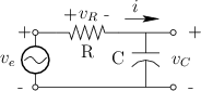
Figure E.1 shows a simple analog filter consisting of one resistor
(![]() Ohms) and one capacitor (
Ohms) and one capacitor (![]() Farads). The voltages across these
elements are
Farads). The voltages across these
elements are ![]() and
and ![]() , respectively, where
, respectively, where ![]() denotes
time in seconds. The filter input is the externally applied voltage
denotes
time in seconds. The filter input is the externally applied voltage
![]() , and the filter output is taken to be
, and the filter output is taken to be ![]() . By
Kirchoff's loop constraints [20], we have
. By
Kirchoff's loop constraints [20], we have
and the loop current is
Capacitors
A capacitor can be made physically using two parallel conducting plates which are held close together (but not touching). Electric charge can be stored in a capacitor by applying a voltage across the plates.
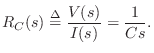
The defining equation of a capacitor ![]() is
is
where
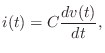
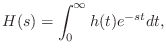
Taking the Laplace transform of both sides gives
Assuming a zero initial voltage across the capacitor at time 0, we have
Mechanical Equivalent of a Capacitor is a Spring
The mechanical analog of a capacitor is the compliance of a
spring. The voltage ![]() across a capacitor
across a capacitor ![]() corresponds to the
force
corresponds to the
force ![]() used to displace a spring. The charge
used to displace a spring. The charge ![]() stored in
the capacitor corresponds to the displacement
stored in
the capacitor corresponds to the displacement ![]() of the spring.
Thus, Eq.
of the spring.
Thus, Eq.![]() (E.2) corresponds to Hooke's law for ideal springs:
(E.2) corresponds to Hooke's law for ideal springs:
Inductors
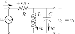
An inductor can be made physically using a coil of wire, and it
stores magnetic flux when a current flows through it. Figure E.2
shows a circuit in which a resistor ![]() is in series with the parallel
combination of a capacitor
is in series with the parallel
combination of a capacitor ![]() and inductor
and inductor ![]() .
.
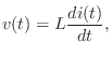
The defining equation of an inductor ![]() is
is
where
where
Taking the Laplace transform of both sides gives
Assuming a zero initial current in the inductor at time 0, we have
Mechanical Equivalent of an Inductor is a Mass
The mechanical analog of an inductor is a mass. The voltage
![]() across an inductor
across an inductor ![]() corresponds to the force
corresponds to the force ![]() used to
accelerate a mass
used to
accelerate a mass ![]() . The current
. The current ![]() through in the inductor
corresponds to the velocity
through in the inductor
corresponds to the velocity
![]() of the mass. Thus,
Eq.
of the mass. Thus,
Eq.![]() (E.4) corresponds to Newton's second law for an ideal mass:
(E.4) corresponds to Newton's second law for an ideal mass:
From the defining equation ![]() for an inductor [Eq.
for an inductor [Eq.![]() (E.3)], we
see that the stored magnetic flux in an inductor is analogous to mass
times velocity, or momentum. In other words, magnetic flux may
be regarded as electric-charge momentum.
(E.3)], we
see that the stored magnetic flux in an inductor is analogous to mass
times velocity, or momentum. In other words, magnetic flux may
be regarded as electric-charge momentum.
RC Filter Analysis
Referring again to Fig.E.1, let's perform an impedance analysis of the simple RC lowpass filter.
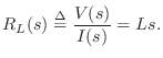
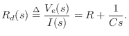
Driving Point Impedance
Taking the Laplace transform of both sides of Eq.![]() (E.1) gives
(E.1) gives
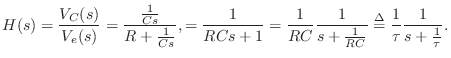
Transfer Function
Since the input and output signals are defined as ![]() and
and
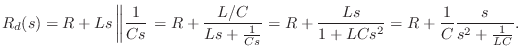
![]() , respectively, the transfer function of this analog
filter is given by, using voltage divider rule,
, respectively, the transfer function of this analog
filter is given by, using voltage divider rule,
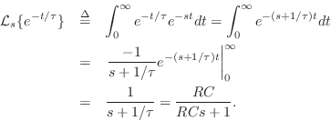
Impulse Response
In the same way that the impulse response of a digital filter is given by the inverse z transform of its transfer function, the impulse response of an analog filter is given by the inverse Laplace transform of its transfer function, viz.,
![$\displaystyle u(t) \isdef \left\{\begin{array}{ll}
1, & t\geq 0 \\ [5pt]
0, & t<0. \\
\end{array}\right.
$](http://www.dsprelated.com/josimages_new/filters/img1814.png)
In more complicated situations, any rational ![]() (ratio of
polynomials in
(ratio of
polynomials in ![]() ) may be expanded into first-order terms by means of
a partial fraction expansion (see §6.8) and each term in
the expansion inverted by inspection as above.
) may be expanded into first-order terms by means of
a partial fraction expansion (see §6.8) and each term in
the expansion inverted by inspection as above.
The Continuous-Time Impulse
The continuous-time impulse response was derived above as the inverse-Laplace transform of the transfer function. In this section, we look at how the impulse itself must be defined in the continuous-time case.
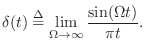
An impulse in continuous time may be loosely defined as any ``generalized function'' having ``zero width'' and unit area under it. A simple valid definition is
![$\displaystyle \delta(t) \isdef \lim_{\Delta \to 0} \left\{\begin{array}{ll} \fr...
...eq t\leq \Delta \\ [5pt] 0, & \hbox{otherwise}. \\ \end{array} \right. \protect$](http://www.dsprelated.com/josimages_new/filters/img1818.png)
More generally, an impulse can be defined as the limit of any pulse shape which maintains unit area and approaches zero width at time 0. As a result, the impulse under every definition has the so-called sifting property under integration,
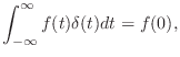
provided
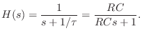
Poles and Zeros
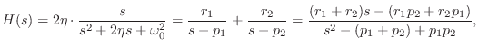
In the simple RC-filter example of §E.4.3, the transfer function is
RLC Filter Analysis
Referring now to Fig.E.2, let's perform an impedance analysis of that RLC network.
Driving Point Impedance
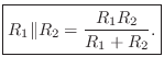
By inspection, we can write
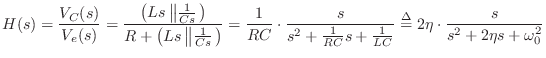
Transfer Function
The transfer function in this example can similarly be found using voltage divider rule:
Poles and Zeros
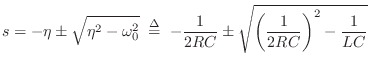
From the quadratic formula, the two poles are located at
Impulse Response
The impulse response is again the inverse Laplace transform of the
transfer function. Expanding ![]() into a sum of complex one-pole
sections,
into a sum of complex one-pole
sections,
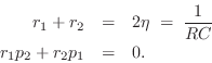
This pair of equations in two unknowns may be solved for ![]() and
and ![]() .
The impulse response is then
.
The impulse response is then
Relating Pole Radius to Bandwidth
Consider the continuous-time complex one-pole
resonator with ![]() -plane transfer function
-plane transfer function
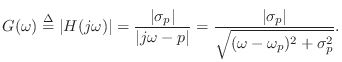
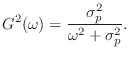
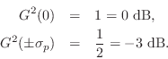
This shows that the 3-dB bandwidth of the resonator in radians
per second is
![]() , or twice the absolute value of the real
part of the pole. Denoting the 3-dB bandwidth in Hz by
, or twice the absolute value of the real
part of the pole. Denoting the 3-dB bandwidth in Hz by ![]() , we have
derived the relation
, we have
derived the relation
![]() , or
, or
It now remains to ``digitize'' the continuous-time resonator and show
that relation Eq.![]() (8.7) follows. The most natural mapping of the
(8.7) follows. The most natural mapping of the
![]() plane to the
plane to the ![]() plane is
plane is
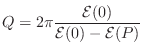
Quality Factor (Q)
The quality factor (Q) of a two-pole resonator is defined by [20, p. 184]
where
Note that Q is defined in the context of continuous-time resonators, so the transfer function
By the quadratic formula, the poles of the transfer function ![]() are given by
are given by
Therefore, the poles are complex only when
Relating to the notation of the previous section, in which we defined
one of the complex poles as
![]() , we have
, we have
| (E.10) | |||
| (E.11) |
For resonators,
Since the imaginary parts of the complex resonator poles are
![]() , the zero-crossing rate of the resonator impulse
response is
, the zero-crossing rate of the resonator impulse
response is
![]() crossings per second. Moreover,
crossings per second. Moreover, ![]() is very close to the peak-magnitude frequency in the resonator
amplitude response. If we eliminate the negative-frequency pole,
is very close to the peak-magnitude frequency in the resonator
amplitude response. If we eliminate the negative-frequency pole,
![]() becomes exactly the peak frequency. In other
words, as a measure of resonance peak frequency,
becomes exactly the peak frequency. In other
words, as a measure of resonance peak frequency, ![]() only
neglects the interaction of the positive- and negative-frequency
resonance peaks in the frequency response, which is usually negligible
except for highly damped, low-frequency resonators. For any amount of
damping
only
neglects the interaction of the positive- and negative-frequency
resonance peaks in the frequency response, which is usually negligible
except for highly damped, low-frequency resonators. For any amount of
damping
![]() gives the impulse-response zero-crossing rate
exactly, as is immediately seen from the derivation in the next
section.
gives the impulse-response zero-crossing rate
exactly, as is immediately seen from the derivation in the next
section.
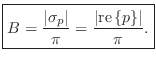
Decay Time is Q Periods
Another well known rule of thumb is that the ![]() of a resonator is the
number of ``periods'' under the exponential decay of its impulse
response. More precisely, we will show that, for
of a resonator is the
number of ``periods'' under the exponential decay of its impulse
response. More precisely, we will show that, for ![]() , the
impulse response decays by the factor
, the
impulse response decays by the factor ![]() in
in ![]() cycles, which
is about 96 percent decay, or -27 dB.
cycles, which
is about 96 percent decay, or -27 dB.
The impulse response corresponding to Eq.![]() (E.8) is found by
inverting the Laplace transform of the transfer function
(E.8) is found by
inverting the Laplace transform of the transfer function ![]() . Since it
is only second order, the solution can be found in many tables of
Laplace transforms. Alternatively, we can break it up into a sum of
first-order terms which are invertible by inspection (possibly after
rederiving the Laplace transform of an exponential decay, which is
very simple). Thus we perform the partial fraction expansion of
Eq.
. Since it
is only second order, the solution can be found in many tables of
Laplace transforms. Alternatively, we can break it up into a sum of
first-order terms which are invertible by inspection (possibly after
rederiving the Laplace transform of an exponential decay, which is
very simple). Thus we perform the partial fraction expansion of
Eq.![]() (E.8) to obtain
(E.8) to obtain
| (E.12) | |||
| (E.13) |
as the respective residues of the poles
The impulse response is thus
Assuming a resonator, ![]() , we have
, we have
![]() , where
, where
![]() (using notation of the
preceding section), and the impulse response reduces to
(using notation of the
preceding section), and the impulse response reduces to
We have shown so far that the impulse response ![]() decays as
decays as
![]() with a sinusoidal radian frequency
with a sinusoidal radian frequency
![]() under the exponential envelope. After Q periods at frequency
under the exponential envelope. After Q periods at frequency
![]() , time has advanced to
, time has advanced to
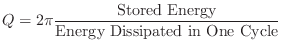
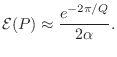
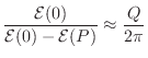
Q as Energy Stored over Energy Dissipated
Yet another meaning for ![]() is as follows [20, p. 326]
is as follows [20, p. 326]
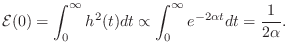
Proof. The total stored energy at time ![]() is
equal to the total energy of the remaining response. After an impulse
at time 0, the stored energy in a second-order resonator is
is
equal to the total energy of the remaining response. After an impulse
at time 0, the stored energy in a second-order resonator is
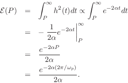
Assuming ![]() as before,
as before,
![]() so that
so that
Analog Allpass Filters
It turns out that analog allpass filters are considerably simpler
mathematically than digital allpass filters (discussed in
§B.2). In fact, when working with digital allpass filters,
it can be fruitful to convert to the analog case using the bilinear
transform (§I.3.1), so that the filter may be manipulated in the
analog ![]() plane rather than the digital
plane rather than the digital ![]() plane. The analog case
is simpler because analog allpass filters may be described as having a
zero at
plane. The analog case
is simpler because analog allpass filters may be described as having a
zero at
![]() for every pole at
for every pole at ![]() , while digital allpass
filters must have a zero at
, while digital allpass
filters must have a zero at
![]() for every pole at
for every pole at ![]() .
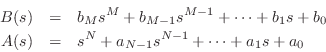
In particular, the transfer function of every first-order analog
allpass filter can be written as
.
In particular, the transfer function of every first-order analog
allpass filter can be written as
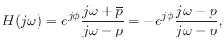
This simplified rule works because every complex pole
Multiplying out the terms in Eq.![]() (E.14), we find that the numerator
polynomial
(E.14), we find that the numerator
polynomial ![]() is simply related to the denominator polynomial
is simply related to the denominator polynomial ![]() :
:
As an example of the greater simplicity of analog allpass filters
relative to the discrete-time case, the graphical method for computing
phase response from poles and zeros (§8.3) gives immediately
that the phase response of every real analog allpass filter is equal
to twice the phase response of its numerator (plus ![]() when
the frequency response is negative at dc). This is because the angle
of a vector from a pole at
when
the frequency response is negative at dc). This is because the angle
of a vector from a pole at ![]() to the point
to the point ![]() along the
frequency axis is
along the
frequency axis is ![]() minus the angle of the vector from a zero at
minus the angle of the vector from a zero at
![]() to the point
to the point ![]() .
.
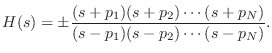
Lossless Analog Filters
As discussed in §B.2, the an allpass filter can be defined
as any filter that preserves signal energy for every input
signal ![]() . In the continuous-time case, this means
. In the continuous-time case, this means
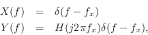
where ![]() denotes the Dirac ``delta function'' or continuous
impulse function (§E.4.3). Thus, the allpass condition becomes
denotes the Dirac ``delta function'' or continuous
impulse function (§E.4.3). Thus, the allpass condition becomes
Suppose

(We have normalized ![]() so that
so that ![]() is monic (
is monic (![]() ) without
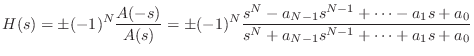
loss of generality.) Equation (E.15) implies
) without
loss of generality.) Equation (E.15) implies
 and
and  , in which case
 for all
  .
.
-
 and , i.e.,
By analytic continuation, we have
Next Section:
Matrix Filter Representations
Previous Section:
Introduction to Laplace Transform Analysis


