


Modal Expansion
A well known approach to transfer-function modeling is called modal synthesis, introduced in §1.3.9 [5,299,6,145,381,30]. Modal synthesis may be defined as constructing a source-filter synthesis model in which the filter transfer function is implemented as a sum of first- and/or second-order filter sections (i.e., as a parallel filter bank in which each filter is at most second-order--this was reviewed in §1.3.9). In other words, the physical system is represented as a superposition of individual modes driven by some external excitation (such as a pluck or strike).
In acoustics, the term mode of vibration, or normal mode, normally refers to a single-frequency spatial eigensolution of the governing wave equation. For example, the modes of an ideal vibrating string are the harmonically related sinusoidal string-shapes having an integer number of uniformly spaced zero-crossings (or nodes) along the string, including its endpoints. As first noted by Daniel Bernoulli (§A.2), acoustic vibration can be expressed as a superposition of component sinusoidal vibrations, i.e., as a superposition of modes.9.6
When a single mode is excited by a sinusoidal driving force, all points of the physical object vibrate at the same temporal frequency (cycles per second), and the mode shape becomes proportional to the spatial amplitude envelope of the vibration. The sound emitted from the top plate of a guitar, for example, can be represented as a weighted sum of the radiation patterns of the respective modes of the top plate, where the weighting function is constructed according to how much each mode is excited (typically by the guitar bridge) [143,390,109,205,209].
The impulse-invariant method (§8.2), can be considered a
special case of modal synthesis in which a continuous-time ![]() -plane
transfer function is given as a starting point. More typically, modal
synthesis starts with a measured frequency response, and a
second-order parallel filter bank is fit to that in some way. In
particular, any filter-design technique may be used (§8.6),
followed by a conversion to second-order parallel form.
-plane
transfer function is given as a starting point. More typically, modal
synthesis starts with a measured frequency response, and a
second-order parallel filter bank is fit to that in some way. In
particular, any filter-design technique may be used (§8.6),
followed by a conversion to second-order parallel form.
Modal expansions find extensive application in industry for determining parametric frequency responses (superpositions of second-order modes) from measured vibration data [299]. Each mode is typically parametrized in terms of its resonant frequency, bandwidth (or damping), and gain (most generally complex gain, to include phase).
Modal synthesis can also be seen as a special case of source-filter synthesis, which may be defined as any signal model based on factoring a sound-generating process into a filter driven by some (usually relatively simple) excitation signal. An early example of source-filter synthesis is the vocoder (§A.6.1). Whenever the filter in a source-filter model is implemented as a parallel second-order filter bank, we can call it modal synthesis (although, strictly speaking, each filter section should correspond to a resonant mode of the modeled resonant system).
Also related to modal synthesis is so-called formant synthesis, used extensively in speech synthesis [219,255,389,40,81,491,490,313,363,297]. A formant is simply a filter resonance having some center-frequency, bandwidth, and (sometimes specified) gain. Thus, a formant corresponds to a single mode of vibration in the vocal tract. Many text-to-speech systems in use today are based on the Klatt formant synthesizer for speech [255].
Since the importance of spectral formants in sound synthesis has more to do with the way we hear than with the physical parameters of a system, formant synthesis is probably best viewed as a spectral modeling synthesis method [456], as opposed to a physical modeling technique [435]. An exception to this rule may occur when the system consists physically of a parallel bank of second-order resonators, such as an array of tuning forks or Helmholtz resonators. In such a case, the mode parameters correspond to physically independent objects; this is of course rare in practice.
In the linear, time-invariant case, only modes in the range of human hearing need to be retained in the model. Also, any ``uncontrollable'' or ``unobservable'' modes should obviously be left out as well. With these simplificiation, the modal representation is generally more efficient than an explicit mass-spring-dashpot digitization (§7.3). On the other hand, since the modal representation is usually not directly physical, nonlinear extensions may be difficult and/or behave unnaturally.
As in the impulse-invariant method (§8.2), starting with an
order ![]() transfer function
transfer function ![]() describing the input-output
behavior of a physical system, a modal description can be obtained
immediately from the partial fraction expansion (PFE):
describing the input-output
behavior of a physical system, a modal description can be obtained
immediately from the partial fraction expansion (PFE):
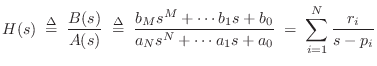
where
 |
(9.10) |
Let
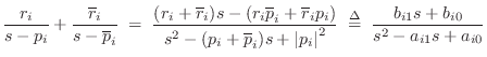
The real poles, if any, can be paired off into a sum of second-order sections as well, with one first-order section left over when
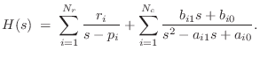
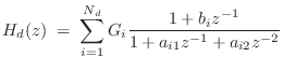
A typical practical implementation of each mode in the sum is by means of second-order filter, or biquad section [449]. A biquad section is easily converted from continuous- to discrete-time form, such as by the impulse-invariant method of §8.2. The final discrete-time model then consist of a parallel bank of second-order digital filters
where
Expressing complex poles of ![]() in polar form as
in polar form as
![]() , (where now we assume
, (where now we assume ![]() denotes a pole in the
denotes a pole in the ![]() plane), we obtain the classical relations [449]
plane), we obtain the classical relations [449]
These parameters are in turn related to the modal parameters resonance frequency
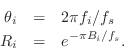
Often ![]() and
and ![]() are estimated from a measured log-magnitude
frequency-response (see §8.8 for a discussion of various methods).
are estimated from a measured log-magnitude
frequency-response (see §8.8 for a discussion of various methods).
It remains to determine the overall section gain ![]() in
Eq.
in
Eq.![]() (8.12), and the coefficient
(8.12), and the coefficient ![]() determining the zero location.
If
determining the zero location.
If ![]() (as is common in practice, since the human ear is not very
sensitive to spectral nulls), then
(as is common in practice, since the human ear is not very
sensitive to spectral nulls), then ![]() can be chosen to match the
measured peak height. A particularly simple automatic method is to
use least-squares minimization to compute
can be chosen to match the
measured peak height. A particularly simple automatic method is to
use least-squares minimization to compute ![]() using Eq.
using Eq.![]() (8.12)
with
(8.12)
with ![]() and
and ![]() fixed (and
fixed (and ![]() ). Generally speaking,
least-squares minimization is always immediate when the error to be
minimized is linear in the unknown parameter (in this case
). Generally speaking,
least-squares minimization is always immediate when the error to be
minimized is linear in the unknown parameter (in this case ![]() ).
).
To estimate ![]() in Eq.
in Eq.![]() (8.12), an effective method is to work
initially with a complex, first-order partial fraction
expansion, and use least squares to determine complex gain
coefficients
(8.12), an effective method is to work
initially with a complex, first-order partial fraction
expansion, and use least squares to determine complex gain
coefficients ![]() for first-order (complex) terms of the form
for first-order (complex) terms of the form
Sections implementing two real poles are not conveniently specified in
terms of resonant frequency and bandwidth. In such cases, it is more
common to work with the filter coefficients ![]() and
and ![]() directly,
as they are often computed by system-identification software
[288,428] or general purpose filter design
utilities, such as in Matlab or Octave [443].
directly,
as they are often computed by system-identification software
[288,428] or general purpose filter design
utilities, such as in Matlab or Octave [443].
To summarize, numerous techniques exist for estimating modal parameters from measured frequency-response data, and some of these are discussed in §8.8 below. Specifically, resonant modes can be estimated from the magnitude, phase, width, and location of peaks in the Fourier transform of a recorded (or estimated) impulse response Another well known technique is Prony's method [449, p. 393], [297]. There is also a large literature on other methods for estimating the parameters of exponentially decaying sinusoids; examples include the matrix-pencil method [274], and parametric spectrum analysis in general [237].
State Space Approach to Modal Expansions
The preceding discussion of modal synthesis was based primarily on fitting a sum of biquads to measured frequency-response peaks. A more general way of arriving at a modal representation is to first form a state space model of the system [449], and then convert to the modal representation by diagonalizing the state-space model. This approach has the advantage of preserving system behavior between the given inputs and outputs. Specifically, the similarity transform used to diagonalize the system provides new input and output gain vectors which properly excite and observe the system modes precisely as in the original system. This procedure is especially more convenient than the transfer-function based approach above when there are multiple inputs and outputs. For some mathematical details, see [449]9.7For a related worked example, see §C.17.6.
Delay Loop Expansion
When a subset of the resonating modes are nearly harmonically tuned, it can be much more computationally efficient to use a filtered delay loop (see §2.6.5) to generate an entire quasi-harmonic series of modes rather than using a biquad for each modal peak [439]. In this case, the resonator model becomes
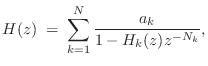
Note that when ![]() is close to
is close to ![]() instead of
instead of ![]() , primarily
only odd harmonic resonances are produced, as has been used in
modeling the clarinet [431].
, primarily
only odd harmonic resonances are produced, as has been used in
modeling the clarinet [431].
Next Section:
Frequency-Response Matching Using Digital Filter Design Methods
Previous Section:
Pole Mapping with Optimal Zeros


