Scattering at Impedance Changes

Free Books Physical Audio Signal Processing

When a traveling wave encounters a change in wave impedance, scattering occurs, i.e., a traveling wave impinging on an impedance discontinuity will partially reflect and partially transmit at the junction in such a way that energy is conserved. This is a classical topic in transmission line theory [295], and it is well covered for acoustic tubes in a variety of references [297,363]. However, for completeness, we derive the basic scattering relations below for plane waves in air, and for longitudinal stress waves in rods.

Plane-Wave Scattering

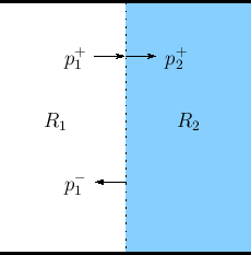
**Figure C.15:** Plane wave propagation in a medium changing from wave impedance to .
$\includegraphics{eps/planewavescat}$

Consider a plane wave with peak pressure amplitude propagating from wave impedance into a new wave impedance , as shown in Fig.C.15. (Assume and are real and positive.) The physical constraints on the wave are that

pressure must be continuous everywhere, and
velocity in must equal velocity out (the junction has no state).

Since power is pressure times velocity, these constraints imply that signal power is conserved at the junction.^C.5Expressed mathematically, the physical constraints at the junction can be written as follows:

$\begin{eqnarray*} p^+_1+p^-_1 &=& p^+_2\quad\mbox{(pressure continuous across ju... ...+}_1+v^{-}_1 &=& v^{+}_2\quad\mbox{(velocity in = velocity out)} \end{eqnarray*}$

As derived in §C.7.3, we also have the Ohm's law relations:

$\begin{displaymath} \begin{array}{rcrl} p^+_i&=&&R_iv^{+}_i\\ p^-_i&=&-&R_iv^{-}_i \end{array}\end{displaymath}$

These equations determine what happens at the junction.

To obey the physical constraints at the impedance discontinuity, the incident plane-wave must split into a reflected plane wave and a transmitted plane-wave such that pressure is continuous and signal power is conserved. The physical pressure on the left of the junction is , and the physical pressure on the right of the junction is , since according to our set-up.

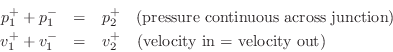
Scattering Solution

Define the junction pressure and junction velocity by

$\begin{eqnarray*} p_j &\isdef & p^+_1+p^-_1 = p^+_2\quad\mbox{(pressure at junct... ...f & v^{+}_1+v^{-}_1 = v^{+}_2\quad\mbox{(velocity at junction).} \end{eqnarray*}$

Then we can write

$\begin{eqnarray*} p^+_1+p^-_1 &=& p^+_2\;=\;p_j\\ [10pt] \,\,\Rightarrow\,\,R_1v... ...\\ [10pt] \,\,\Rightarrow\,\,2\,R_1v^{+}_1 - R_1 v_j &=& R_2 v_j \end{eqnarray*}$

$\displaystyle \,\,\Rightarrow\,\,\zbox {v_j = \frac{2\,R_1}{R_1 + R_2}v^{+}_1.}$

Note that $v_j=v^{+}_2$ , so we have found the velocity of the transmitted wave. Since $v_j = v^{+}_1+v^{-}_1$ , the velocity of the reflected wave is simply

$\displaystyle v^{-}_1 = v_j - v^{+}_1 = \left[\frac{2\,R_1}{R_1+R_2} - 1\right]v^{+}_1 = \frac{R_1-R_2}{R_1+R_2} v^{+}_1.$

We have solved for the transmitted and reflected velocity waves given the incident wave and the two impedances.

Using the Ohm's law relations, the pressure waves follow easily:

$\begin{eqnarray*} p^+_2 &=& R_2v^{+}_2 = R_2 v_j = \frac{2\,R_2}{R_1+R_2}p^+_1\\ [10pt] p^-_1 &=& -R_1v^{-}_1 = \frac{R_2-R_1}{R_1+R_2} p^+_1 \end{eqnarray*}$

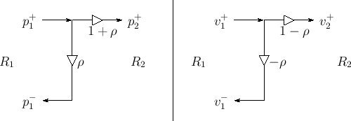
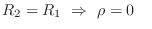
Reflection Coefficient

Define the reflection coefficient of the scattering junction as

$\displaystyle \zbox {\rho = \frac{R_2-R_1}{R_1+R_2} = \frac{\mbox{Impedance Step}}{\mbox{Impedance Sum}}.}$

Then we get the following scattering relations in terms of $\rho$ for pressure waves:

$\begin{eqnarray*} p^+_2 &=& (1+\rho)p^+_1\\ [3pt] p^-_1 &=& \rho\,p^+_1 \end{eqnarray*}$

Signal flow graphs for pressure and velocity are given in Fig.C.16.

**Figure C.16:** Signal flow graph for the pressure and velocity components of a plane wave scattering at an impedance discontinuity :.
$\includegraphics{eps/planewavescatdm2}$

It is a simple exercise to verify that signal power is conserved by checking that $p^+_1v^{+}_1 = p^+_2v^{+}_2 + ( - p^-_1v^{-}_1)$ . (Left-going power is negated to account for its opposite direction-of-travel.)

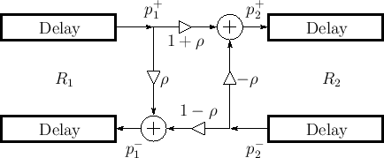
So far we have only considered a plane wave incident on the left of the junction. Consider now a plane wave incident from the right. For that wave, the impedance steps from to , so the reflection coefficient it ``sees'' is $-\rho$ . By superposition, the signal flow graph for plane waves incident from either side is given by Fig.C.17. Note that the transmission coefficient is one plus the reflection coefficient in either direction. This signal flow graph is often called the ``Kelly-Lochbaum'' scattering junction [297].

**Figure C.17:** Signal flow graph for plane waves incident on either the left or right of an impedance discontinuity. Also shown are delay lines corresponding to sampled traveling plane-wave components propagating on either side of the scattering junction.
$\includegraphics{eps/planewavescatdmfull}$

There are some simple special cases:

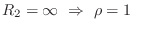$R_2=\infty\,\,\Rightarrow\,\,\rho = 1\quad$ (e.g., rigid wall reflection)
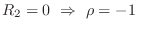$R_2=0\,\,\Rightarrow\,\,\rho = -1\quad$ (e.g., open-ended tube)
$R_2=R_1\,\,\Rightarrow\,\,\rho = 0\quad$ (no reflection)

Plane-Wave Scattering at an Angle

Figure C.18 shows the more general situation (as compared to Fig.C.15) of a sinusoidal traveling plane wave encountering an impedance discontinuity at some arbitrary angle of incidence, as indicated by the vector wavenumber $\underline{k}_1^+$ . The mathematical details of general sinusoidal plane waves in air and vector wavenumber are reviewed in §B.8.1.

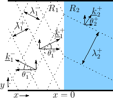**Figure C.18:** Sinusoidal plane wave scattering at an impedance discontinuity--oblique angle of incidence $\theta _1^+$ .
$\includegraphics{eps/planewavescatangle}$

At the boundary between impedance and , we have, by continuity of pressure,

$\begin{eqnarray*} k_1\sin(\theta_1^+) &=&k_1\sin(\theta_1^-) \;=\;k_2\sin(\theta_2^+) \end{eqnarray*}$

as we will now derive.

Let the impedance change be in the $\underline{x}=(0,y,z)$ plane. Thus, the impedance is for $x\le0$ and for . There are three plane waves to consider:

The incident plane wave with wave vector $\underline{k}_1^+$
The reflected plane wave with wave vector $\underline{k}_1^-$
The transmitted plane wave with wave vector $\underline{k}_2^+$

By continuity, the waves must agree on boundary plane:

$\displaystyle \left<\underline{k}_1^+,\underline{r}\right> = \left<\underline{k}_1^-,\underline{r}\right> = \left<\underline{k}_2^+,\underline{r}\right>$

where $\underline{r}=(0,y,z)$ denotes any vector in the boundary plane. Thus, at

we have

$\displaystyle k_{1y}^+\,y + k_{1z}^+\,z = k_{1y}^-\,y + k_{1z}^-\,z = k_{2y}^+\,y + k_{2z}^+\,z.$

If the incident wave is constant along

, then $k_{1z}^+=0$ , requiring $k_{1z}^- = k_{2z}^+ = 0$ , leaving

$\displaystyle k_{1y}^+\,y = k_{1y}^-\,y =k_{2y}^+\,y$

$\displaystyle \zbox {k_1\sin(\theta_1^+) =k_1\sin(\theta_1^-) =k_2\sin(\theta_2^+)} \protect$

(C.56)

where $\theta$ is defined as zero when traveling in the direction of positive

for the incident ( $\underline{k}_1^+$ ) and transmitted ( $\underline{k}_2^+$ ) wave vector, and along negative

for the reflected ( $\underline{k}_1^-$ ) wave vector (see Fig.C.18).

Reflection and Refraction

The first equality in Eq. $\,$ (C.56) implies that the angle of incidence equals angle of reflection:

$\displaystyle \zbox {\theta_1^+=\theta_1^-} % \isdef\theta_1}$

We now wish to find the wavenumber in medium 2. Let denote the phase velocity in wave impedance :

$\displaystyle c_i = \frac{\omega}{k_i}, \quad i=1,2$

In impedance

, we have in particular

$\displaystyle \omega^2 \eqsp c_2^2 k_2^2 \eqsp c_2^2 \left[(k^+_{2x})^2 + (k^+_{2y})^2\right].$

Solving for $k^+_{2x}$ gives

$\displaystyle k^+_{2x} \eqsp \sqrt{\frac{\omega^2}{c_2^2} - (k^+_{2y})^2} \eqsp \sqrt{\frac{\omega^2}{c_2^2} - k_2^2\sin^2(\theta_2^+)}.$

Since $k_1\sin(\theta_1^+)=k_2\sin(\theta_2^+)$ from above,

$\displaystyle k^+_{2x} \eqsp \sqrt{\frac{\omega^2}{c_2^2} - k_1^2\sin^2(\theta... ...\eqsp \sqrt{\frac{\omega^2}{c_2^2}-\frac{\omega^2}{c_1^2}\sin^2(\theta_1^+)}.$

We have thus derived

$\displaystyle \zbox {k^+_{2x} \eqsp \frac{\omega}{c_2}\sqrt{1 - \frac{c_2^2}{c_1^2}\sin^2(\theta_1^+)}.}$

We earlier established $k^+_{2y} = k^+_{1y}$ (for agreement along the boundary, by pressure continuity). This describes the refraction of the plane wave as it passes through the impedance-change boundary. The refraction angle depends on ratio of phase velocities

. This ratio is often called the index of refraction:

$\displaystyle n \isdef \frac{c_2}{c_1}$

and the relation $k_1\sin(\theta_1^+)=k_2\sin(\theta_2^+)$ is called Snell's Law (of refraction).

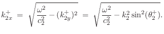
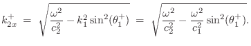
Evanescent Wave due to Total Internal Reflection

Note that if $c_1 < c_2 \vert\sin(\theta_1^+)\vert$ , the horizontal component of the wavenumber in medium 2 becomes imaginary. In this case, the wave in medium 2 is said to be evanescent, and the wave in medium 1 undergoes total internal reflection (no power travels from medium 1 to medium 2). The evanescent-wave amplitude decays exponentially to the right and oscillates ``in place'' (like a standing wave). ``Tunneling'' is possible given a medium 3 beyond medium 2 in which wave propagation resumes.

To show explicitly the exponential decay and in-place oscillation in an evanescent wave, express the imaginary wavenumber as $k_x\isdef -j\kappa_x$ . Then we have

$\begin{eqnarray*} p(t,\underline{x}) &=& \cos\left(\omega t - \underline{k}^T\... ...-k_x x}\right\}}}\\ [5pt] &=& e^{-k_x x} \cos(\omega t - k_y y). \end{eqnarray*}$

Thus, an imaginary wavenumber corresponds to an exponentially decaying evanescent wave. Note that the time dependence (cosine term) applies to all points to the right of the boundary. Since evanescent waves do not really ``propagate,'' it is perhaps better to speak of an ``evanescent acoustic field'' or ``evanescent standing wave'' instead of ``evanescent waves''.

For more on the physics of evanescent waves and tunneling, see [295].

Longitudinal Waves in Rods

In this section, elementary scattering relations will be derived for the case of longitudinal force and velocity waves in an ideal string or rod. In solids, force-density waves are referred to as stress waves [169,261]. Longitudinal stress waves in strings and rods have units of (compressive) force per unit area and are analogous to longitudinal pressure waves in acoustic tubes.

**Figure:** A waveguide section between two partial sections. a) Physical picture indicating traveling waves in a continuous medium whose wave impedance changes from to to . b) Digital simulation diagram for the same situation. The section propagation delay is denoted as $z^{-T}$ . The behavior at an impedance discontinuity is characterized by a lossless splitting of an incoming wave into transmitted and reflected components.
$\includegraphics[width=\twidth]{eps/Fwgfs}$

A single waveguide section between two partial sections is shown in Fig.C.19. The sections are numbered 0 through from left to right, and their wave impedances are , , and , respectively. Such a rod might be constructed, for example, using three different materials having three different densities. In the th section, there are two stress traveling waves: $f^{{+}}_i$ traveling to the right at speed , and $f^{{-}}_i$ traveling to the left at speed . To minimize the numerical dynamic range, velocity waves may be chosen instead when .

As in the case of transverse waves (see the derivation of (C.46)), the traveling longitudinal plane waves in each section satisfy [169,261]

$\begin{displaymath}\begin{array}{rcrl} f^{{+}}_i(t)&=&&R_iv^{+}_i(t) \\ f^{{-}}_i(t)&=&-&R_iv^{-}_i(t) \end{array}\end{displaymath}$

(C.57)

where the wave impedance is now $R_i=\sqrt{E\rho}$ , with $\rho$ being the mass density, and

being the Young's modulus of the medium (defined as the stress over the strain, where strain means relative displacement--see §B.5.1) [169,261]. As before, velocity $v_i=v^{+}_i+v^{-}_i$ is defined as positive to the right, and $f^{{+}}_i$ is the right-going traveling-wave component of the stress, and it is positive when the rod is locally compressed.

If the wave impedance is constant, the shape of a traveling wave is not altered as it propagates from one end of a rod-section to the other. In this case we need only consider $f^{{+}}_i$ and $f^{{-}}_i$ at one end of each section as a function of time. As shown in Fig.C.19, we define $f^\pm _i(t)$ as the force-wave component at the extreme left of section . Therefore, at the extreme right of section , we have the traveling waves $f^{{+}}_i(t-T)$ and $f^{{-}}_i(t+T)$ , where is the travel time from one end of a section to the other.

For generality, we may allow the wave impedances to vary with time. A number of possibilities exist which satisfy (C.57) in the time-varying case. For the moment, we will assume the traveling waves at the extreme right of section are still given by $f^{{+}}_i(t-T)$ and $f^{{-}}_i(t+T)$ . This definition, however, implies the velocity varies inversely with the wave impedance. As a result, signal energy, being the product of force times velocity, is ``pumped'' into or out of the waveguide by a changing wave impedance. Use of normalized waves $\tilde{f}^\pm _i$ avoids this. However, normalization increases the required number of multiplications, as we will see in §C.8.6 below.

As before, the physical force density (stress) and velocity at the left end of section are obtained by summing the left- and right-going traveling wave components:

$\displaystyle f_i$	$\displaystyle =$	$\displaystyle f^{{+}}_i+ f^{{-}}_i$	(C.58)
$\displaystyle v_i$	$\displaystyle =$	$\displaystyle v^{+}_i+ v^{-}_i$

Let

denote the force at position

and time

in section

, where $x_i\in[0,cT]$ is measured from the extreme left of section

along its axis. Then we have, for example, $f_i(t,0)\isdef f^{{+}}_i(t)+f^{{-}}_i(t)$ and $f_i(t,cT)\isdef f^{{+}}_i(t-T)+f^{{-}}_i(t+T)$ at the boundaries of section

. More generally, within section

, the physical stress may be expressed in terms of its traveling-wave components by

$\displaystyle f_i(t,x_i) \eqsp f^{{+}}_i\left(t-\frac{x_i}{c}\right)+f^{{-}}_i\left(t+\frac{x_i}{c}\right), \quad 0\leq x_i\leq cT.$

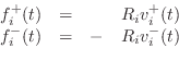
Kelly-Lochbaum Scattering Junctions

Conservation of energy and mass dictate that, at the impedance discontinuity, force and velocity variables must be continuous

$\displaystyle f_{i-1}(t,cT)$	$\displaystyle =$	$\displaystyle f_i(t,0)$	(C.59)
$\displaystyle v_{i-1}(t,cT)$	$\displaystyle =$	$\displaystyle v_i(t,0)$

where velocity is defined as positive to the right on both sides of the junction. Force (or stress or pressure) is a scalar while velocity is a vector with both a magnitude and direction (in this case only left or right). Equations (C.57), (C.58), and (C.59) imply the following scattering equations (a derivation is given in the next section for the more general case of

waveguides meeting at a junction):

$\displaystyle f^{{+}}_i(t)$	$\displaystyle =$	$\displaystyle \left[1+k_i(t) \right]f^{{+}}_{i-1}(t-T) - k_i(t) f^{{-}}_i(t)$
$\displaystyle f^{{-}}_{i-1}(t+T)$	$\displaystyle =$	$\displaystyle k_i(t)f^{{+}}_{i-1}(t-T) + \left[1-k_i(t)\right]f^{{-}}_i(t)$	(C.60)

where

$\displaystyle k_i(t) \isdef \frac{ R_i(t)-R_{i-1}(t) }{R_i(t)+R_{i-1}(t) }$

(C.61)

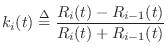
is called the

th reflection coefficient. Since $R_i(t)\geq 0$ , we have $k_i(t)\in[-1,1]$ . It can be shown that if $\vert k_i\vert>1$ , then either

or $R_{i-1}$ is negative, and this implies an active (as opposed to passive) medium. Correspondingly, lattice and ladder recursive digital filters are stable if and only if all reflection coefficients are bounded by

in magnitude [297].

**Figure C.20:** The Kelly-Lochbaum scattering junction.
$\includegraphics[scale=0.9]{eps/Fkl}$

The scattering equations are illustrated in Figs. C.19b and C.20. In linear predictive coding of speech [482], this structure is called the Kelly-Lochbaum scattering junction, and it is one of several types of scattering junction used to implement lattice and ladder digital filter structures (§C.9.4,[297]).

One-Multiply Scattering Junctions

By factoring out in each equation of (C.60), we can write

$\displaystyle f^{{+}}_i(t)$	$\displaystyle =$	$\displaystyle f^{{+}}_{i-1}(t-T) + f_{{\Delta}}(t)$
$\displaystyle f^{{-}}_{i-1}(t+T)$	$\displaystyle =$	$\displaystyle f^{{-}}_i(t) + f_{{\Delta}}(t)$	(C.62)

where

$\displaystyle f_{{\Delta}}(t) \isdef k_i(t)\left[f^{{+}}_{i-1}(t-T) - f^{{-}}_i(t) \right]$

(C.63)

Thus, only one multiplication is actually necessary to compute the transmitted and reflected waves from the incoming waves in the Kelly-Lochbaum junction. This computation is shown in Fig.C.21, and it is known as the one-multiply scattering junction [297].

**Figure C.21:** The one-multiply scattering junction.
$\includegraphics[scale=0.9]{eps/Fom}$

Another one-multiply form is obtained by organizing (C.60) as

$\displaystyle f^{{+}}_i(t)$	$\displaystyle =$	$\displaystyle f^{{-}}_i(t) + \alpha_i(t)\tilde{f_d}(t)$
$\displaystyle f^{{-}}_{i-1}(t+T)$	$\displaystyle =$	$\displaystyle f^{{+}}_i(t) - \tilde{f_d}(t)$	(C.64)

where

$\displaystyle \alpha_i(t)$	$\displaystyle \isdef$	$\displaystyle 1+k_i(t)$
$\displaystyle \tilde{f_d}(t)$	$\displaystyle \isdef$	$\displaystyle f^{{+}}_{i-1}(t-T) - f^{{-}}_i(t).$	(C.65)

As in the previous case, only one multiplication and three additions are required per junction. This one-multiply form generalizes more readily to junctions of more than two waveguides, as we'll see in a later section.

A scattering junction well known in the LPC speech literature but not described here is the so-called two-multiply junction [297] (requiring also two additions). This omission is because the two-multiply junction is not valid as a general, local, physical modeling building block. Its derivation is tied to the reflectively terminated, cascade waveguide chain. In cases where it applies, however, it can be the implementation of choice; for example, in DSP chips having a fast multiply-add instruction, it may be possible to implement the inner loop of the two-multiply, two-add scattering junction using only two instructions.

Normalized Scattering Junctions

**Figure C.22:** The normalized scattering junction.
$\includegraphics[scale=0.9]{eps/scatnlf}$

Using (C.53) to convert to normalized waves $\tilde{f}^\pm$ , the Kelly-Lochbaum junction (C.60) becomes

$\displaystyle \tilde{f}^{+}_i(t)$	$\displaystyle =$	$\displaystyle \sqrt{1-k_i^2(t)}\, \tilde{f}^{+}_{i-1}(t-T) - k_i(t)\, \tilde{f}^{-}_i(t)$
$\displaystyle \tilde{f}^{-}_{i-1}(t+T)$	$\displaystyle =$	$\displaystyle k_i(t)\,\tilde{f}^{+}_{i-1}(t-T) + \sqrt{1-k_i^2(t)}\,\tilde{f}^{-}_i(t)$	(C.66)

as diagrammed in Fig.C.22. This is called the normalized scattering junction [297], although a more precise term would be the ``normalized-wave scattering junction.''

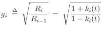
It is interesting to define $\theta_i \isdef \sin^{-1}(k_i)$ , always possible for passive junctions since $-1\leq k_i\leq 1$ , and note that the normalized scattering junction is equivalent to a 2D rotation:

$\displaystyle \tilde{f}^{+}_i(t)$	$\displaystyle =$	$\displaystyle \cos(\theta_i) \, \tilde{f}^{+}_{i-1}(t-T) - \sin(\theta_i) \, \tilde{f}^{-}_i(t)$
$\displaystyle \tilde{f}^{-}_{i-1}(t+T)$	$\displaystyle =$	$\displaystyle \sin(\theta_i)\, \tilde{f}^{+}_{i-1}(t-T) + \cos(\theta_i)\, \tilde{f}^{-}_i(t)$	(C.67)

where, for conciseness of notation, the time-invariant case is written.

While it appears that scattering of normalized waves at a two-port junction requires four multiplies and two additions, it is possible to convert this to three multiplies and three additions using a two-multiply ``transformer'' to power-normalize an ordinary one-multiply junction [432].

The transformer is a lossless two-port defined by [136]

$\displaystyle f^{{+}}_i(t)$	$\displaystyle =$	$\displaystyle g_i\, f^{{+}}_{i-1}(t-T)$
$\displaystyle f^{{-}}_{i-1}(t+T)$	$\displaystyle =$	$\displaystyle \frac{1}{g_i}\,f^{{-}}_i(t).$	(C.68)

The transformer can be thought of as a device which steps the wave impedance to a new value without scattering; instead, the traveling signal power is redistributed among the force and velocity wave variables to satisfy the fundamental relations $f^\pm =\pm Rv^\pm$ (C.57) at the new impedance. An impedance change from $R_{i-1}$ on the left to

on the right is accomplished using

$\displaystyle g_i \isdefs \sqrt\frac{R_i}{R_{i-1}} \eqsp \sqrt\frac{1+k_i(t)}{1-k_i(t)} \protect$

(C.69)

as can be quickly derived by requiring $(f^{{+}}_{i-1})^2/R_{i-1}= (f^{{+}}_i)^2/R_i$ . The parameter

can be interpreted as the ``turns ratio'' since it is the factor by which force is stepped (and the inverse of the velocity step factor).

**Figure C.23:** Three-multiply normalized-wave scattering junction.
$\includegraphics{eps/scatThreeMulNLFx}$

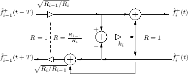
Figure C.23 illustrates a three-multiply normalized-wave scattering junction [432]. The impedance of all waveguides (bidirectional delay lines) may be taken to be . Scattering junctions may then be implemented as a denormalizing transformer $g=\sqrt{R_{i-1}}$ , a one-multiply scattering junction , and a renormalizing transformer $g=1/\sqrt{R_i}$ . Either transformer may be commuted with the junction and combined with the other transformer to give a three-multiply normalized-wave scattering junction. (The transformers are combined on the left in Fig.C.23).

In slightly more detail, a transformer $g=\sqrt{R_{i-1}}$ steps the wave impedance (left-to-right) from to $R=R_{i-1}$ . Equivalently, the normalized force-wave $\tilde{f}^{+}_{i-1}(t)$ is converted unnormalized form $f^{{+}}_{i-1}(t)$ . Next there is a physical scattering from impedance $R_{i-1}$ to (reflection coefficient $k_i=(R_i-R_{i-1})/(R_i+R_{i-1})$ ). The outgoing wave to the right is then normalized by transformer $g=1/\sqrt{R_i}$ to return the wave impedance back to for wave propagation within a normalized-wave delay line to the right. Finally, the right transformer is commuted left and combined with the left transformer to reduce total computational complexity to one multiply and three adds.

It is important to notice that transformer-normalized junctions may have a large dynamic range in practice. For example, if $k_i\in [-1+\epsilon,1-\epsilon]$ , then Eq. $\,$ (C.69) shows that the transformer coefficients may become as large as $\sqrt{2/\epsilon - 1}$ . If $\epsilon$ is the ``machine epsilon,'' i.e., $\epsilon = 2^{-(n-1)}$ for typical -bit two's complement arithmetic normalized to lie in , then the dynamic range of the transformer coefficients is bounded by $\sqrt{2^n-1}\approx 2^{n/2}$ . Thus, while transformer-normalized junctions trade a multiply for an add, they require up to % more bits of dynamic range within the junction adders. On the other hand, it is very nice to have normalized waves (unit wave impedance) throughout the digital waveguide network, thereby limiting the required dynamic range to root physical power in all propagation paths.

Junction Passivity

In fixed-point implementations, the round-off error and other nonlinear operations should be confined when possible to physically meaningful wave variables. When this is done, it is easy to ensure that signal power is not increased by the nonlinear operations. In other words, nonlinear operations such as rounding can be made passive. Since signal power is proportional to the square of the wave variables, all we need to do is make sure amplitude is never increased by the nonlinearity. In the case of rounding, magnitude truncation, sometimes called ``rounding toward zero,'' is one way to achieve passive rounding. However, magnitude truncation can attenuate the signal excessively in low-precision implementations and in scattering-intensive applications such as the digital waveguide mesh [518]. Another option is error power feedback in which case the cumulative round-off error power averages to zero over time.

A valuable byproduct of passive arithmetic is the suppression of limit cycles and overflow oscillations [432]. Formally, the signal power of a conceptually infinite-precision implementation can be taken as a Lyapunov function bounding the squared amplitude of the finite-precision implementation.

The Kelly-Lochbaum and one-multiply scattering junctions are structurally lossless [500,460] (see also §C.17) because they have only one parameter (or $\alpha_i$ ), and all quantizations of the parameter within the allowed interval (or ) correspond to lossless scattering.^C.6

In the Kelly-Lochbaum and one-multiply scattering junctions, because they are structurally lossless, we need only double the number of bits at the output of each multiplier, and add one bit of extended dynamic range at the output of each two-input adder. The final outgoing waves are thereby exactly computed before they are finally rounded to the working precision and/or clipped to the maximum representable magnitude.

For the Kelly-Lochbaum scattering junction, given -bit signal samples and -bit reflection coefficients, the reflection and transmission multipliers produce and bits, respectively, and each of the two additions adds one more bit. Thus, the intermediate word length required is bits, and this must be rounded without amplification down to bits for the final outgoing samples. A similar analysis gives also that the one-multiply scattering junction needs bits for the extended precision intermediate results before final rounding and/or clipping.

To formally show that magnitude truncation is sufficient to suppress overflow oscillations and limit cycles in waveguide networks built using structurally lossless scattering junctions, we can look at the signal power entering and leaving the junction. A junction is passive if the power flowing away from it does not exceed the power flowing into it. The total power flowing away from the th junction is bounded by the incoming power if

$\displaystyle \underbrace{\frac{[f^{{+}}_i(t)]^2}{R_i(t)} + \frac{[f^{{-}}_{i-1... ...t-T)]^2}{R_{i-1}(t)} + \frac{[f^{{-}}_i(t)]^2}{R_i(t)}}_{\mbox{incoming power}}$

(C.70)

Let ${\hat f}$ denote the finite-precision version of

. Then a sufficient condition for junction passivity is

$\displaystyle \left\vert{\hat f}^{+}_i(t)\right\vert$	$\displaystyle \leq$	$\displaystyle \left\vert f^{{+}}_i(t)\right\vert$	(C.71)
$\displaystyle \left\vert{\hat f}^{-}_{i-1}(t+T)\right\vert$	$\displaystyle \leq$	$\displaystyle \left\vert f^{{-}}_{i-1}(t+T)\right\vert$	(C.72)

Thus, if the junction computations do not increase either of the output force amplitudes, no signal power is created. An analogous conclusion is reached for velocity scattering junctions.

Unlike the structurally lossless cases, the (four-multiply) normalized scattering junction has two parameters, $s_i\isdeftext k_i$ and $c_i\isdeftext \sqrt{1-k_i^2}$ , and these can ``get out of synch'' in the presence of quantization. Specifically, let ${\hat s}_i \isdeftext s_i - \epsilon_s$ denote the quantized value of , and let ${\hat c}_i\isdeftext c_i -\epsilon_c$ denote the quantized value of . Then it is no longer the case in general that ${\hat s}^2_i + {\hat c}^2_i= 1$ . As a result, the normalized scattering junction is not structurally lossless in the presence of coefficient quantization. A few lines of algebra shows that a passive rounding rule for the normalized junction must depend on the sign of the wave variable being computed, the sign of the coefficient quantization error, and the sign of at least one of the two incoming traveling waves. We can assume one of the coefficients is exact for passivity purposes, so assume $\epsilon_s=0$ and define ${\hat c}_i=\left\lfloor \sqrt{1-s^2_i}\right\rfloor$ , where $\left\lfloor x\right\rfloor$ denotes largest quantized value less than or equal to . In this case we have $\epsilon_c\geq 0$ . Therefore,

$\displaystyle {\hat f}^{+}_i= {\hat c}_if^{{+}}_{i-1}- s_i f^{{-}}_i= f^{{+}}_i- \epsilon_c f^{{+}}_{i-1}$

and a passive rounding rule which guarantees $\vert{\hat f}^{+}_i\vert \leq \vert f^{{+}}_i\vert$ need only look at the sign bits of ${\hat f}^{+}_i$ and $f^{{+}}_{i-1}$ .

The three-multiply normalized scattering junction is easier to ``passify.'' While the transformer is not structurally lossless, its simplicity allows it to be made passive simply by using non-amplifying rounding on both of its coefficients as well as on its output wave variables. (The transformer is passive when the product of its coefficients has magnitude less than or equal to .) Since there are no additions following the transformer multiplies, double-precision adders are not needed. However, precision and a half is needed in the junction adders to accommodate the worst-case increased dynamic range. Since the one-multiply junction is structurally lossless, the overall junction is passive if non-amplifying rounding is applied to , , and the outgoing wave variables from the transformer and from the one-multiply junction.

In summary, a general means of obtaining passive waveguide junctions is to compute exact results internally, and apply saturation (clipping on overflow) and magnitude truncation (truncation toward zero) to the final outgoing wave variables. Because the Kelly-Lochbaum and one-multiply junctions are structurally lossless, exact intermediate results are obtainable using extended internal precision. For the (four-multiply) normalized scattering junction, a passive rounding rule can be developed based on two sign bits. For the three-multiply normalized scattering junction, it is sufficient to apply magnitude truncation to the transformer coefficients and all outgoing wave variables.

Next Section:
Digital Waveguide Filters
Previous Section:
Alternative Wave Variables