


Electric Guitars
For electric guitars, which are mainly about the vibrating string and subsequent effects processing, we pick up where §6.7 left off, and work our way up to practical complexity step by step. We begin with practical enhancements for the waveguide string model that are useful for all kinds of guitar models.
Length Three FIR Loop Filter
The simplest nondegenerate example of the loop filters of §6.8
is the three-tap FIR case (
![]() ). The symmetry constraint
leaves two degrees of freedom in the frequency response:10.1
). The symmetry constraint
leaves two degrees of freedom in the frequency response:10.1
Length  FIR Loop Filter Controlled by ``Brightness'' and ``Sustain''
Another convenient parametrization of the second-order symmetric FIR
case is when the dc normalization is relaxed so that two degrees of
freedom are retained. It is then convenient to control them
as brightness ![]() and sustain
and sustain ![]() according to the
formulas
according to the
formulas
where
One-Zero Loop Filter
If we relax the constraint that
![]() be odd, then the simplest case
becomes the one-zero digital filter:
be odd, then the simplest case
becomes the one-zero digital filter:
See [454] for related discussion from a software implementation perspective.
The Karplus-Strong Algorithm
The simulation diagram for the ideal string with the simplest frequency-dependent loss filter is shown in Fig. 9.1. Readers of the computer music literature will recognize this as the structure of the Karplus-Strong algorithm [236,207,489].
![\includegraphics[width=\twidth]{eps/fkarplusstrong}](http://www.dsprelated.com/josimages_new/pasp/img1962.png) |
The Karplus-Strong algorithm, per se, is obtained when the
delay-line initial conditions used to ``pluck'' the string consist of
random numbers, or ``white noise.'' We know the initial shape
of the string is obtained by adding the upper and lower delay
lines of Fig. 6.11, i.e.,
![]() . It is shown in §C.7.4 that the initial
velocity distribution along the string is determined by the
difference between the upper and lower delay lines. Thus, in
the Karplus-Strong algorithm, the string is ``plucked'' by a
random initial displacement and initial velocity distribution.
This is a very energetic excitation, and usually in practice the white
noise is lowpass filtered; the lowpass cut-off frequency gives an
effective dynamic level control since natural stringed
instruments are typically brighter at louder dynamic levels
[428,207].
. It is shown in §C.7.4 that the initial
velocity distribution along the string is determined by the
difference between the upper and lower delay lines. Thus, in
the Karplus-Strong algorithm, the string is ``plucked'' by a
random initial displacement and initial velocity distribution.
This is a very energetic excitation, and usually in practice the white
noise is lowpass filtered; the lowpass cut-off frequency gives an
effective dynamic level control since natural stringed
instruments are typically brighter at louder dynamic levels
[428,207].
Karplus-Strong sound examples are available on the Web.
An implementation of the Karplus-Strong algorithm in the Faust programming language is described (and provided) in [454].
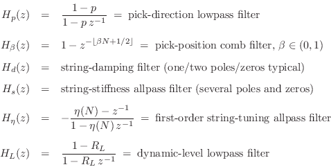
The Extended Karplus-Strong Algorithm
Figure 9.2 shows a block diagram of the Extended Karplus-Strong (EKS) algorithm [207].
![\includegraphics[width=\twidth]{eps/eks}](http://www.dsprelated.com/josimages_new/pasp/img1964.png)
The EKS adds the following features to the KS algorithm:
where
Note that while
![]() can be used in the tuning allpass, it
is better to offset it to
can be used in the tuning allpass, it
is better to offset it to
![]() to avoid delays
close to zero in the tuning allpass. (A zero delay is obtained by a
pole-zero cancellation on the unit circle.) First-order allpass
interpolation of delay lines was discussed in §4.1.2.
to avoid delays
close to zero in the tuning allpass. (A zero delay is obtained by a
pole-zero cancellation on the unit circle.) First-order allpass
interpolation of delay lines was discussed in §4.1.2.
A history of the Karplus-Strong algorithm and its extensions is given
in §A.8. EKS sound
examples
are also available on the Web. Techniques for designing the
string-damping filter ![]() and/or the string-stiffness allpass
filter
and/or the string-stiffness allpass
filter ![]() are summarized below in §6.11.
are summarized below in §6.11.
An implementation of the Extended Karplus-Strong (EKS) algorithm in the Faust programming language is described (and provided) in [454].
Nonlinear Distortion
In §6.13, nonlinear elements were introduced in the context of general digital waveguide synthesis. In this section, we discuss specifically virtual electric guitar distortion, and mention other instances of audible nonlinearity in stringed musical instruments.
As discussed in Chapter 6, typical vibrating strings in musical acoustics are well approximated as linear, time-invariant systems, there are special cases in which nonlinear behavior is desired.
Tension Modulation
In every freely vibrating string, the fundamental frequency declines
over time as the amplitude of vibration decays. This is due to
tension modulation, which is often audible at the beginning of
plucked-string tones, especially for low-tension strings. It happens
because higher-amplitude vibrations stretch the string to a
longer average length, raising the average string tension
![]() faster wave propagation
faster wave propagation
![]() higher fundamental
frequency.
higher fundamental
frequency.
The are several methods in the literature for simulating tension modulation in a digital waveguide string model [494,233,508,512,513,495,283], as well as in membrane models [298]. The methods can be classified into two categories, local and global.
Local tension-modulation methods modulate the speed of sound locally as a function of amplitude. For example, opposite delay cells in a force-wave digital waveguide string can be summed to obtain the instantaneous vertical force across that string sample, and the length of the adjacent propagation delay can be modulated using a first-order allpass filter. In principle the string slope reduces as the local tension increases. (Recall from Chapter 6 or Appendix C that force waves are minus the string tension times slope.)
Global tension-modulation methods [495,494] essentially modulate the string delay-line length as a function of the total energy in the string.
String Length Modulation
A number of stringed musical instruments have a ``nonlinear sound'' that comes from modulating the physical termination of the string (as opposed to its acoustic length in the case of tension modulation).
The Finnish Kantele [231,513] has a different effective string-length in the vertical and horizontal vibration planes due to a loose knot attaching the string to a metal bar. There is also nonlinear feeding of the second harmonic due to a nonrigid tuning peg.
Perhaps a better known example is the Indian sitar, in which a curved ``jawari'' (functioning as a nonlinear bridge) serves to shorten the string gradually as it displaces toward the bridge.
The Indian tambura also employs a thread perpendicular to the strings a short distance from the bridge, which serves to shorten the string whenever string displacement toward the bridge exceeds a certain distance.
Finally, the slap bass playing technique for bass guitars involves hitting the string hard enough to cause it to beat against the neck during vibration [263,366].
In all of these cases, the string length is physically modulated in some manner each period, at least when the amplitude is sufficiently large.
Hard Clipping
A widespread class of distortion used in electric guitars, is clipping of the guitar waveform. it is easy to add this effect to any string-simulation algorithm by passing the output signal through a nonlinear clipping function. For example, a hard clipper has the characteristic (in normalized form)
![$\displaystyle f(x) = \left\{\begin{array}{ll} -1, & x\leq -1 \\ [5pt] x, & -1 \leq x \leq 1 \\ [5pt] 1, & x\geq 1 \\ \end{array} \right. \protect$](http://www.dsprelated.com/josimages_new/pasp/img1514.png)
where
Soft Clipping
A soft clipper is similar to a hard clipper, but with the corners smoothed. A common choice of soft-clipper is the cubic nonlinearity, e.g. [489],
![$\displaystyle f(x) = \left\{\begin{array}{ll} -\frac{2}{3}, & x\leq -1 \\ [5pt]...
... \leq x \leq 1 \\ [5pt] \frac{2}{3}, & x\geq 1. \\ \end{array} \right. \protect$](http://www.dsprelated.com/josimages_new/pasp/img1970.png)
This particular soft-clipping characteristic is diagrammed in Fig.9.3. An analysis of its spectral characteristics, with some discussion of aliasing it may cause, was given in in §6.13. An input gain may be used to set the desired degree of distortion.
![\includegraphics[width=3in]{eps/cnl}](http://www.dsprelated.com/josimages_new/pasp/img1971.png)
Enhancing Even Harmonics
A cubic nonlinearity, as well as any odd distortion law,10.2 generates only odd-numbered harmonics (like in a square wave). For best results, and in particular for tube distortion simulation [31,395], it has been argued that some amount of even-numbered harmonics should also be present. Breaking the odd symmetry in any way will add even-numbered harmonics to the output as well. One simple way to accomplish this is to add an offset to the input signal, obtaining
Another method for breaking the odd symmetry is to add some square-law nonlinearity to obtain
where
Software for Cubic Nonlinear Distortion
The function cubicnl in the Faust software distribution (file effect.lib) implements cubic nonlinearity distortion [454]. The Faust programming example cubic_distortion.dsp provides a real-time demo with adjustable parameters, including an offset for bringing in even harmonics. The free, open-source guitarix application (for Linux platforms) uses this type of distortion effect along with many other guitar effects.
In the Synthesis Tool Kit (STK) [91], the class Cubicnl.cpp implements a general cubic distortion law.
Amplifier Feedback
A more extreme effect used with distorted electric guitars is amplifier feedback. In this case, the amplified guitar waveforms couple back to the strings with some gain and delay, as depicted schematically in Fig.9.4 [489].
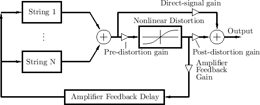
The Amplifier Feedback Delay in the figure can be adjusted to
emphasize certain partial overtones over others. If the loop gain,
controllable via the Amplifier Feedback Gain, is greater than 1 at any
frequency, a sustained ``feedback howl'' will be
produced. Note that in commercial devices, the Pre-distortion gain
and Post-distortion gain are frequency-dependent, i.e., they are
implemented as pre- and post-equalizers (typically only a few
bands, such as three). Another simple choice is an integrator
![]() for the pre-distortion gain, and a differentiator
for the pre-distortion gain, and a differentiator
![]() for the post-distortion gain.
for the post-distortion gain.
Faust software implementing electric-guitar amplifier feedback may be found in [454].
Cabinet Filtering
The distortion output signal is often further filtered by an amplifier cabinet filter, representing the enclosure, driver responses, etc. It is straightforward to measure the impulse response (or frequency response) of a speaker cabinet and fit it with a recursive digital filter design function such as invfreqz in matlab (§8.6.4). Individual speakers generally have one major resonance--the ``cone resonance''--which is determined by the mass, compliance, and damping of the driver subassembly. The enclosing cabinet introduces many more resonances in the audio range, generally tuned to even out the overall response as much as possible.
Faust software implementing an idealized speaker filter may be found in [454].
Duty-Cycle Modulation
For class A tube amplifier simulation, there should be level-dependent duty-cycle modulation as a function:10.3
- 50% at low amplitude levels (no duty-cycle modulation)
- 55-65% duty cycle at high levels
Vacuum Tube Modeling
The elementary nonlinearities discussed above are aimed at approximating the sound of amplifier distortion, such as often used by guitar players. Generally speaking, the distortion characteristics of vacuum-tube amplifiers are considered superior to those of solid-state amplifiers. A real-time numerically solved nonlinear differential algebraic model for class A single-ended guitar power amplification is presented in [84]. Real-time simulation of a tube guitar-amp (triode preamp, inverter, and push-pull amplifier) based on a precomputed approximate solution of the nonlinear differential equations is presented in [293]. Other references in this area include [338,228,339].
Next Section:
Acoustic Guitars
Previous Section:
Virtual Analog Example: Phasing


