


The Dispersive 1D Wave Equation
In the ideal vibrating string, the only restoring force for transverse displacement comes from the string tension (§C.1 above); specifically, the transverse restoring force is equal the net transverse component of the axial string tension. Consider in place of the ideal string a bundle of ideal strings, such as a stranded cable. When the cable is bent, there is now a new restoring force arising from some of the fibers being compressed and others being stretched by the bending. This force sums with that due to string tension. Thus, stiffness in a vibrating string introduces a new restoring force proportional to bending angle. It is important to note that string stiffness is a linear phenomenon resulting from the finite diameter of the string.
In typical treatments,C.3bending stiffness adds a new term to the wave equation that is proportional to the fourth spatial derivative of string displacement:
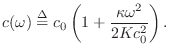
where the moment constant
To solve the stiff wave equation Eq.![]() (C.32),
we may set
(C.32),
we may set
![]() to get
to get
At very high frequencies, or when the tension ![]() is negligible relative
to
is negligible relative
to
![]() , we obtain the ideal bar (or rod) approximation:
, we obtain the ideal bar (or rod) approximation:
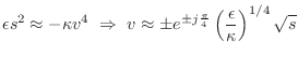
At intermediate frequencies, between the ideal string and the ideal bar,
the stiffness contribution can be treated as a correction term
[95]. This is the region of most practical interest because
it is the principal operating region for strings, such as piano strings,
whose stiffness has audible consequences (an inharmonic, stretched overtone
series). Assuming
![]() ,
,
 |
|||
 |
|||
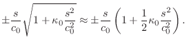 |
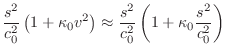
Substituting for
![$\displaystyle e^{st+vx} = \exp{\left\{{s\left[t\pm \frac{x}{c_0}\left(
1+\frac{1}{2}\kappa_0 \frac{s^2}{c_0^2} \right)\right]}\right\}}.
$](http://www.dsprelated.com/josimages_new/pasp/img3398.png)
Since the temporal and spatial sampling intervals are related by ![]() , this must generalize to
, this must generalize to
![]() , where
, where ![]() is the size of a unit
delay in the absence of stiffness. Thus, a unit delay
is the size of a unit
delay in the absence of stiffness. Thus, a unit delay ![]() may be
replaced by
may be
replaced by
![\includegraphics[scale=0.9]{eps/fstiffstring}](http://www.dsprelated.com/josimages_new/pasp/img3406.png)
The general, order ![]() , allpass filter is given by [449]
, allpass filter is given by [449]
For computability of the string simulation in the presence of scattering
junctions, there must be at least one sample of pure delay along each
uniform section of string. This means for at least one allpass filter in
Fig.C.8, we must have
![]() which
implies
which
implies ![]() can be factored as
can be factored as
![]() . In a
systolic VLSI implementation, it is desirable to have at least one real
delay from the input to the output of every allpass filter, in order
to be able to pipeline the computation of all of the allpass filters in
parallel. Computability can be arranged in practice by deciding on a
minimum delay, (e.g., corresponding to the wave velocity at a maximum
frequency), and using an allpass filter to provide excess delay beyond the
minimum.
. In a
systolic VLSI implementation, it is desirable to have at least one real
delay from the input to the output of every allpass filter, in order
to be able to pipeline the computation of all of the allpass filters in
parallel. Computability can be arranged in practice by deciding on a
minimum delay, (e.g., corresponding to the wave velocity at a maximum
frequency), and using an allpass filter to provide excess delay beyond the
minimum.
Because allpass filters are linear and time invariant, they commute
like gain factors with other linear, time-invariant components.
Fig.C.9 shows a diagram equivalent to
Fig.C.8 in which the allpass filters have been
commuted and consolidated at two points. For computability in all
possible contexts (e.g., when looped on itself), a single sample of
delay is pulled out along each rail. The remaining transfer function,
![]() in the example of
Fig.C.9, can be approximated using any allpass filter
design technique
[1,2,267,272,551].
Alternatively, both gain and dispersion for a stretch of waveguide can
be provided by a single filter which can be designed using any
general-purpose filter design method which is sensitive to
frequency-response phase as well as magnitude; examples include
equation error methods (such as used in the matlab invfreqz
function (§8.6.4), and Hankel norm methods
[177,428,36].
in the example of
Fig.C.9, can be approximated using any allpass filter
design technique
[1,2,267,272,551].
Alternatively, both gain and dispersion for a stretch of waveguide can
be provided by a single filter which can be designed using any
general-purpose filter design method which is sensitive to
frequency-response phase as well as magnitude; examples include
equation error methods (such as used in the matlab invfreqz
function (§8.6.4), and Hankel norm methods
[177,428,36].
![\includegraphics[scale=0.9]{eps/flstiffstring}](http://www.dsprelated.com/josimages_new/pasp/img3413.png) |
In the case of a lossless, stiff string, if ![]() denotes the
consolidated allpass transfer function, it can be argued that the filter
design technique used should minimize the phase-delay error, where
phase delay is defined by [362]
denotes the
consolidated allpass transfer function, it can be argued that the filter
design technique used should minimize the phase-delay error, where
phase delay is defined by [362]
 (Phase Delay)
Alternatively, a lumped allpass filter can be designed by minimizing group delay,
 (Group Delay)
See §9.4.1 for designing allpass filters with a prescribed delay versus frequency. To model stiff strings, the allpass filter must supply a phase delay which decreases as frequency increases. A good approximation may require a fairly high-order filter, adding significantly to the cost of simulation. (For low-pitched piano strings, order 8 allpass filters work well perceptually [1].) To a large extent, the allpass order required for a given error tolerance increases as the number of lumped frequency-dependent delays is increased. Therefore, increased dispersion consolidation is accompanied by larger required allpass filters, unlike the case of resistive losses.
The function piano_dispersion_filter in the Faust distribution (in effect.lib) designs and implements an allpass filter modeling the dispersion due to stiffness in a piano string [154,170,368].
Higher Order Terms
The complete, linear, time-invariant generalization of the lossy, stiff string is described by the differential equation
which, on setting
 |
(C.34) |
Solving for
| (C.35) | |||
where
We see that a large class of wave equations with constant coefficients, of any order, admits a decaying, dispersive, traveling-wave type solution. Even-order time derivatives give rise to frequency-dependent dispersion and odd-order time derivatives correspond to frequency-dependent losses. The corresponding digital simulation of an arbitrarily long (undriven and unobserved) section of medium can be simplified via commutativity to at most two pure delays and at most two linear, time-invariant filters.
Every linear, time-invariant filter can be expressed as a zero-phase filter in series with an allpass filter. The zero-phase part can be interpreted as implementing a frequency-dependent gain (damping in a digital waveguide), and the allpass part can be seen as frequency-dependent delay (dispersion in a digital waveguide).
Next Section:
Alternative Wave Variables
Previous Section:
A Lossy 1D Wave Equation


