


Derivation of the Discrete Fourier Transform (DFT)
This chapter derives the Discrete Fourier Transform (DFT) as a
projection of a length ![]() signal
signal ![]() onto the set of
onto the set of ![]() sampled
complex sinusoids generated by the
sampled
complex sinusoids generated by the ![]() th roots of unity.
th roots of unity.
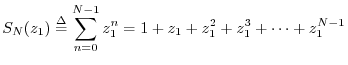
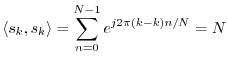
Geometric Series
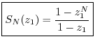
Recall that for any complex number
![]() , the signal
, the signal
Proof: We have
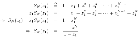
When ![]() ,
, ![]() , by inspection of the definition of
, by inspection of the definition of
![]() .
.
Orthogonality of Sinusoids
A key property of sinusoids is that they are orthogonal at different frequencies. That is,
For length ![]() sampled sinusoidal signal segments, such as used
by the DFT, exact orthogonality holds only for the harmonics of
the sampling-rate-divided-by-
sampled sinusoidal signal segments, such as used
by the DFT, exact orthogonality holds only for the harmonics of
the sampling-rate-divided-by-![]() , i.e., only for the frequencies (in Hz)
, i.e., only for the frequencies (in Hz)

The complex sinusoids corresponding to the frequencies ![]() are
are
Nth Roots of Unity
As introduced in §3.12, the complex numbers
![$\displaystyle \left[W_N^k\right]^N = \left[e^{j\omega_k T}\right]^N
= \left[e^{j k 2\pi/N}\right]^N = e^{j k 2\pi} = 1.
$](http://www.dsprelated.com/josimages_new/mdft/img1010.png)
The ![]() th roots of unity are plotted in the complex plane in
Fig.6.1 for
th roots of unity are plotted in the complex plane in
Fig.6.1 for ![]() . It is easy to find them graphically
by dividing the unit circle into
. It is easy to find them graphically
by dividing the unit circle into ![]() equal parts using
equal parts using ![]() points, with
one point anchored at
points, with
one point anchored at ![]() , as indicated in Fig.6.1. When
, as indicated in Fig.6.1. When
![]() is even, there will be a point at
is even, there will be a point at ![]() (corresponding to a sinusoid
with frequency at exactly half the sampling rate), while if
(corresponding to a sinusoid
with frequency at exactly half the sampling rate), while if ![]() is
odd, there is no point at
is
odd, there is no point at ![]() .
.
![\includegraphics[width=\twidth]{eps/dftfreqs}](http://www.dsprelated.com/josimages_new/mdft/img1016.png)
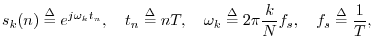
DFT Sinusoids
The sampled sinusoids generated by integer powers of the ![]() roots of
unity are plotted in Fig.6.2. These are the sampled sinusoids
roots of
unity are plotted in Fig.6.2. These are the sampled sinusoids
![]() used by the
DFT. Note that taking successively higher integer powers of the
point
used by the
DFT. Note that taking successively higher integer powers of the
point ![]() on the unit circle
generates samples of the
on the unit circle
generates samples of the ![]() th DFT sinusoid, giving
th DFT sinusoid, giving ![]() ,
,
![]() . The
. The ![]() th sinusoid generator
th sinusoid generator ![]() is in turn
the
is in turn
the ![]() th
th ![]() th root of unity (
th root of unity (![]() th power of the primitive
th power of the primitive ![]() th root
of unity
th root
of unity ![]() ).
).
![\includegraphics[width=\twidth]{eps/dftsines}](http://www.dsprelated.com/josimages_new/mdft/img1019.png)
Note that in Fig.6.2 the range of ![]() is taken to be
is taken to be
![]() instead of
instead of
![]() . This is the most
``physical'' choice since it corresponds with our notion of ``negative
frequencies.'' However, we may add any integer multiple of
. This is the most
``physical'' choice since it corresponds with our notion of ``negative
frequencies.'' However, we may add any integer multiple of ![]() to
to ![]() without changing the sinusoid indexed by
without changing the sinusoid indexed by ![]() . In other words,
. In other words, ![]() refers to the same sinusoid
refers to the same sinusoid
![]() for all integers
for all integers
![]() .
.
Orthogonality of the DFT Sinusoids
We now show mathematically that the DFT sinusoids are exactly orthogonal. Let
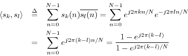
where the last step made use of the closed-form expression for the sum
of a geometric series (§6.1). If ![]() , the
denominator is nonzero while the numerator is zero. This proves
, the
denominator is nonzero while the numerator is zero. This proves
Norm of the DFT Sinusoids
For ![]() , we follow the previous derivation to the next-to-last step to get
, we follow the previous derivation to the next-to-last step to get
An Orthonormal Sinusoidal Set
We can normalize the DFT sinusoids to obtain an orthonormal set:
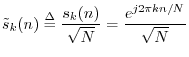
![$\displaystyle \left<\tilde{s}_k,\tilde{s}_l\right> = \left\{\begin{array}{ll}
1, & k=l \\ [5pt]
0, & k\neq l. \\
\end{array} \right.
$](http://www.dsprelated.com/josimages_new/mdft/img1034.png)
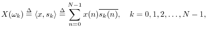
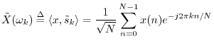
The Discrete Fourier Transform (DFT)
Given a signal
![]() , its DFT is defined
by6.3
, its DFT is defined
by6.3


In summary, the DFT is proportional to the set of coefficients of projection onto the sinusoidal basis set, and the inverse DFT is the reconstruction of the original signal as a superposition of its sinusoidal projections. This basic ``architecture'' extends to all linear orthogonal transforms, including wavelets, Fourier transforms, Fourier series, the discrete-time Fourier transform (DTFT), and certain short-time Fourier transforms (STFT). See Appendix B for some of these.
We have defined the DFT from a geometric signal theory point of view, building on the preceding chapter. See §7.1.1 for notation and terminology associated with the DFT.
Frequencies in the ``Cracks''
The DFT is defined only for frequencies
![]() . If we
are analyzing one or more periods of an exactly periodic signal, where the
period is exactly
. If we
are analyzing one or more periods of an exactly periodic signal, where the
period is exactly ![]() samples (or some integer divisor of
samples (or some integer divisor of ![]() ), then these
really are the only frequencies present in the signal, and the spectrum is
actually zero everywhere but at
), then these
really are the only frequencies present in the signal, and the spectrum is
actually zero everywhere but at
![]() ,
,
![]() .
However, we use the
DFT to analyze arbitrary signals from nature. What happens when a
frequency
.
However, we use the
DFT to analyze arbitrary signals from nature. What happens when a
frequency ![]() is present in a signal
is present in a signal ![]() that is not one of the
DFT-sinusoid frequencies
that is not one of the
DFT-sinusoid frequencies ![]() ?
?
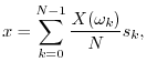
To find out, let's project a length ![]() segment of a sinusoid at an
arbitrary frequency
segment of a sinusoid at an
arbitrary frequency ![]() onto the
onto the ![]() th DFT sinusoid:
th DFT sinusoid:
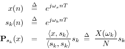
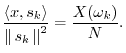
The coefficient of projection is proportional to
![\begin{eqnarray*}
X(\omega_k) & \isdef & \left<x,s_k\right> \;\isdef \; \sum_{n=...
...ac{\sin[(\omega_x-\omega_k)NT/2]}{\sin[(\omega_x-\omega_k)T/2]},
\end{eqnarray*}](http://www.dsprelated.com/josimages_new/mdft/img1048.png)
using the closed-form expression for a geometric series sum once
again. As shown in §6.3-§6.4 above,
the sum is ![]() if
if
![]() and zero at
and zero at ![]() , for
, for ![]() . However,
the sum is nonzero at all other frequencies
. However,
the sum is nonzero at all other frequencies ![]() .
.
Since we are only looking at ![]() samples, any sinusoidal segment can be
projected onto the
samples, any sinusoidal segment can be
projected onto the ![]() DFT sinusoids and be reconstructed exactly by a
linear combination of them. Another way to say this is that the DFT
sinusoids form a basis for
DFT sinusoids and be reconstructed exactly by a
linear combination of them. Another way to say this is that the DFT
sinusoids form a basis for ![]() , so that any length
, so that any length ![]() signal
whatsoever can be expressed as a linear combination of them. Therefore, when
analyzing segments of recorded signals, we must interpret what we see
accordingly.
signal
whatsoever can be expressed as a linear combination of them. Therefore, when
analyzing segments of recorded signals, we must interpret what we see
accordingly.
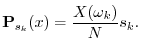
The typical way to think about this in practice is to consider the DFT
operation as a digital filter for each ![]() , whose input is
, whose input is ![]() and whose output is
and whose output is
![]() at time
at time ![]() .6.4 The
frequency response of this filter is what we just
computed,6.5 and its magnitude is
.6.4 The
frequency response of this filter is what we just
computed,6.5 and its magnitude is
![$\displaystyle \left\vert X(\omega_k)\right\vert =
\left\vert\frac{\sin[(\omega_x-\omega_k)NT/2]}{\sin[(\omega_x-\omega_k)T/2]}\right\vert
$](http://www.dsprelated.com/josimages_new/mdft/img1054.png)
![\includegraphics[width=\twidth]{eps/dftfilter}](http://www.dsprelated.com/josimages_new/mdft/img1059.png) |
We see that
![]() is sensitive to all frequencies between dc
and the sampling rate except the other DFT-sinusoid frequencies
is sensitive to all frequencies between dc
and the sampling rate except the other DFT-sinusoid frequencies
![]() for
for ![]() . This is sometimes called spectral leakage
or cross-talk in the spectrum analysis. Again, there is no
leakage when the signal being analyzed is truly periodic and we can choose
. This is sometimes called spectral leakage
or cross-talk in the spectrum analysis. Again, there is no
leakage when the signal being analyzed is truly periodic and we can choose
![]() to be exactly a period, or some multiple of a period. Normally,
however, this cannot be easily arranged, and spectral leakage can
be a problem.
to be exactly a period, or some multiple of a period. Normally,
however, this cannot be easily arranged, and spectral leakage can
be a problem.
Note that peak spectral leakage is not reduced by increasing
![]() .6.7 It can be thought of as being caused by abruptly
truncating a sinusoid at the beginning and/or end of the
.6.7 It can be thought of as being caused by abruptly
truncating a sinusoid at the beginning and/or end of the
![]() -sample time window. Only the DFT sinusoids are not cut off at the
window boundaries. All other frequencies will suffer some truncation
distortion, and the spectral content of the abrupt cut-off or turn-on
transient can be viewed as the source of the sidelobes. Remember
that, as far as the DFT is concerned, the input signal
-sample time window. Only the DFT sinusoids are not cut off at the
window boundaries. All other frequencies will suffer some truncation
distortion, and the spectral content of the abrupt cut-off or turn-on
transient can be viewed as the source of the sidelobes. Remember
that, as far as the DFT is concerned, the input signal ![]() is the
same as its
periodic extension (more about this in
§7.1.2). If we repeat
is the
same as its
periodic extension (more about this in
§7.1.2). If we repeat ![]() samples of a sinusoid at frequency
samples of a sinusoid at frequency
![]() (for any
(for any
![]() ), there will be a ``glitch''
every
), there will be a ``glitch''
every ![]() samples since the signal is not periodic in
samples since the signal is not periodic in ![]() samples.
This glitch can be considered a source of new energy over the entire
spectrum. See
Fig.8.3 for an example waveform.
samples.
This glitch can be considered a source of new energy over the entire
spectrum. See
Fig.8.3 for an example waveform.
To reduce spectral leakage (cross-talk from far-away
frequencies), we typically use a
window
function, such as a
``raised cosine'' window, to taper the data record gracefully
to zero at both endpoints of the window. As a result of the smooth
tapering, the main lobe widens and the sidelobes
decrease in the DFT response. Using no window is better viewed as
using a rectangular window of length ![]() , unless the signal is
exactly periodic in
, unless the signal is
exactly periodic in ![]() samples. These topics are considered further
in Chapter 8.
samples. These topics are considered further
in Chapter 8.
Spectral Bin Numbers
Since the ![]() th spectral sample
th spectral sample
![]() is properly regarded as
a measure of spectral amplitude over a range of frequencies,
nominally
is properly regarded as
a measure of spectral amplitude over a range of frequencies,
nominally ![]() to
to ![]() , this range is sometimes called a
frequency bin
(as in a ``storage bin'' for spectral energy).
The frequency index
, this range is sometimes called a
frequency bin
(as in a ``storage bin'' for spectral energy).
The frequency index ![]() is called the bin number, and
is called the bin number, and
![]() can be regarded as the total energy in the
can be regarded as the total energy in the ![]() th
bin (see §7.4.9).
Similar remarks apply to samples of any
bandlimited
function; however, the term ``bin'' is only used in the frequency
domain, even though it could be assigned exactly the same meaning
mathematically in the time domain.
th
bin (see §7.4.9).
Similar remarks apply to samples of any
bandlimited
function; however, the term ``bin'' is only used in the frequency
domain, even though it could be assigned exactly the same meaning
mathematically in the time domain.
Fourier Series Special Case
In the very special case of truly periodic signals
![]() , for all
, for all
![]() , the DFT may be regarded as
computing the Fourier series coefficients of
, the DFT may be regarded as
computing the Fourier series coefficients of ![]() from one
period of its sampled representation
from one
period of its sampled representation ![]() ,
,
![]() . The
period of
. The
period of ![]() must be exactly
must be exactly ![]() seconds for this to work. For the
details, see §B.3.
seconds for this to work. For the
details, see §B.3.
Normalized DFT
A more ``theoretically clean'' DFT is obtained by projecting onto the normalized DFT sinusoids (§6.5)

It can be said that only the NDFT provides a proper change of
coordinates from the time-domain (shifted impulse basis signals) to
the frequency-domain (DFT sinusoid basis signals). That is, only the
NDFT is a pure
rotation in ![]() , preserving both orthogonality and the unit-norm
property of the basis functions. The DFT, in contrast, preserves
orthogonality, but the norms of the basis functions grow to
, preserving both orthogonality and the unit-norm
property of the basis functions. The DFT, in contrast, preserves
orthogonality, but the norms of the basis functions grow to
![]() . Therefore, in the present context, the DFT coefficients can be
considered ``denormalized'' frequency-domain coordinates.
. Therefore, in the present context, the DFT coefficients can be
considered ``denormalized'' frequency-domain coordinates.
The Length 2 DFT
The length ![]() DFT is particularly simple, since the basis sinusoids
are real:
DFT is particularly simple, since the basis sinusoids
are real:
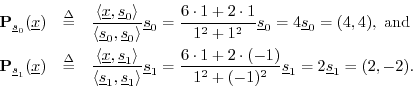
The DFT sinusoid ![]() is a sampled constant signal, while
is a sampled constant signal, while ![]() is a
sampled sinusoid at half the sampling rate.
is a
sampled sinusoid at half the sampling rate.
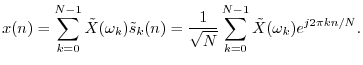
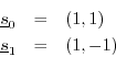
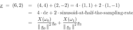
Figure 6.4 illustrates the graphical relationships for the length
![]() DFT of the signal
DFT of the signal
![]() .
.
![\includegraphics[width=\twidth]{eps/dft2}](http://www.dsprelated.com/josimages_new/mdft/img1077.png)
Analytically, we compute the DFT to be
and the corresponding projections onto the DFT sinusoids are
Note the lines of orthogonal projection illustrated in the figure. The
``time domain'' basis consists of the vectors
![]() , and the
orthogonal projections onto them are simply the coordinate axis projections
, and the
orthogonal projections onto them are simply the coordinate axis projections
![]() and
and ![]() . The ``frequency domain'' basis vectors are
. The ``frequency domain'' basis vectors are
![]() , and they provide an orthogonal basis set that is rotated
, and they provide an orthogonal basis set that is rotated
![]() degrees relative to the time-domain basis vectors. Projecting
orthogonally onto them gives
degrees relative to the time-domain basis vectors. Projecting
orthogonally onto them gives
![]() and
and
![]() , respectively.
The original signal
, respectively.
The original signal
![]() can be
expressed either as the vector sum of its coordinate projections
(0,...,x(i),...,0), (a time-domain representation), or as the
vector sum of its projections onto the DFT sinusoids (a
frequency-domain representation of the time-domain signal
can be
expressed either as the vector sum of its coordinate projections
(0,...,x(i),...,0), (a time-domain representation), or as the
vector sum of its projections onto the DFT sinusoids (a
frequency-domain representation of the time-domain signal
![]() ).
Computing the coefficients of projection is essentially ``taking the
DFT,'' and constructing
).
Computing the coefficients of projection is essentially ``taking the
DFT,'' and constructing
![]() as the vector sum of its projections onto
the DFT sinusoids amounts to ``taking the inverse DFT.''
as the vector sum of its projections onto
the DFT sinusoids amounts to ``taking the inverse DFT.''
In summary, the oblique coordinates in Fig.6.4 are interpreted as follows:
Matrix Formulation of the DFT
The DFT can be formulated as a complex matrix multiply, as we show in this section. (This section can be omitted without affecting what follows.) For basic definitions regarding matrices, see Appendix H.
The DFT consists of inner products of the input signal
![]() with sampled complex sinusoidal sections
with sampled complex sinusoidal sections ![]() :
:

![$\displaystyle \underbrace{
\left[\begin{array}{c}
X(\omega_0) \\
X(\omega_1) ...
...
x(2) \\
\vdots \\
x(N-1)
\end{array}\right]
}_{\displaystyle\underline{x}}
$](http://www.dsprelated.com/josimages_new/mdft/img1089.png)
![$\displaystyle \underline{X}= \mathbf{S}^\ast_N \underline{x}
= \left[\begin{arr...
...\ [2pt] \vdots \\ [2pt] \left<\underline{x},\sv_{N-1}\right>\end{array}\right]
$](http://www.dsprelated.com/josimages_new/mdft/img1090.png)
![\begin{eqnarray*}
\mathbf{S}^\ast_N
&\!\!\isdef \!\!& \left[\begin{array}{cccc}...
...-1)/N} & \cdots & e^{-j 2\pi (N-1)(N-1)/N}
\end{array}\!\right].
\end{eqnarray*}](http://www.dsprelated.com/josimages_new/mdft/img1093.png)
The notation
![]() denotes the
Hermitian transpose of the complex matrix
denotes the
Hermitian transpose of the complex matrix ![]() (transposition
and complex conjugation).
(transposition
and complex conjugation).
Note that the ![]() th column of
th column of
![]() is the
is the ![]() th DFT sinusoid, so
that the
th DFT sinusoid, so
that the ![]() th row of the DFT matrix
th row of the DFT matrix
![]() is the
complex-conjugate of the
is the
complex-conjugate of the ![]() th DFT sinusoid. Therefore, multiplying
the DFT matrix times a signal vector
th DFT sinusoid. Therefore, multiplying
the DFT matrix times a signal vector
![]() produces a column-vector
produces a column-vector
![]() in which the
in which the ![]() th element
th element
![]() is the inner
product of the
is the inner
product of the ![]() th DFT sinusoid with
th DFT sinusoid with
![]() , or
, or
![]() , as expected.
, as expected.
Computation of the DFT matrix in Matlab is illustrated in §I.4.3.
The inverse DFT matrix is simply
![]() . That is,
we can perform the inverse DFT operation as
. That is,
we can perform the inverse DFT operation as
Since the forward DFT is
This equation succinctly states that the columns of
![\begin{eqnarray*}
\mathbf{S}^\ast_N \mathbf{S}_N
&\!\!=\!\!&
\left[\!\begin{arr...
...0 & 0 & 0 & \cdots & N
\end{array}\!\right]
= N\cdot \mathbf{I}.
\end{eqnarray*}](http://www.dsprelated.com/josimages_new/mdft/img1105.png)
The normalized DFT matrix is given by
When a real matrix
![]() satisfies
satisfies
![]() , then
, then
![]() is said to be
orthogonal.
``Unitary'' is the generalization of ``orthogonal'' to
complex matrices.
is said to be
orthogonal.
``Unitary'' is the generalization of ``orthogonal'' to
complex matrices.
DFT Problems
See http://ccrma.stanford.edu/~jos/mdftp/DFT_Problems.html
Next Section:
Fourier Theorems for the DFT
Previous Section:
Geometric Signal Theory


