


Spectrum Analysis of Sinusoids
Sinusoidal components are fundamental building blocks of sound. Any sound that can be described as a ``tone'' is naturally and efficiently modeled as a sum of windowed sinusoids over short, ``stationary'' time segments (e.g., on the order of 20 ms or more in the case of voice). Over longer time segments, tonal sounds are modeled efficiently by modulated sinusoids, where the amplitude and frequency modulations are relatively slow. This is the model used in additive synthesis (discussed further below). Of course, thanks to Fourier's theorem, every sound can be expressed as a sum of sinusoids having fixed amplitude and frequency, but this is a highly inefficient model for non-tonal and changing sounds. Perhaps more fundamentally from an audio modeling point of view, the ear is quite sensitive to peaks in the short-time spectrum of a sound, and a spectral peak is naturally modeled as a sinusoidal component which has been shaped by some kind of ``window function'' or ``amplitude envelope'' in the time domain.
Because spectral peaks are so relatively dominant in hearing, sinusoidal models are ``unreasonably effective'' in capturing the tonal aspects of sound in a compact, easy-to-manipulate form. Computing a sinusoidal model entails fitting the parameters of a sinusoid (amplitude, frequency, and sometimes phase) to each peak in the spectrum of each time-segment. In typical sinusoidal modeling systems, the sinusoidal parameters are linearly interpolated from one time segment to the next, and this usually provides a perceptually smooth variation over time. (Higher order interpolation has also been used.) Modeling sound as a superposition of modulated sinusoids in this way is generally called additive synthesis [233].
Additive synthesis is not the only sound modeling method that requires sinusoidal parameter estimation for its calibration to desired signals. For the same reason that additive synthesis is so effective, we routinely calibrate any model for sound production by matching the short-time Fourier transform, and in this matching process, spectral peaks are heavily weighted (especially at low frequencies in the audio range). Furthermore, when the model parameters are few, as in the physical model of a known musical instrument, the model parameters can be determined entirely by the amplitudes and frequencies of the sinusoidal peaks. In such cases, sinusoidal parameter estimation suffices to calibrate non-sinusoidal models.
Pitch detection is another application in which spectral peaks are ``explained'' as harmonics of some estimated fundamental frequency. The harmonic assumption is an example of a signal modeling constraint. Model constraints provide powerful means for imposing prior knowledge about the source of the sound being modeled.
Another application of sinusoidal modeling is source separation. In this case, spectral peaks are measured and tracked over time, and the ones that ``move together'' are grouped together as separate sound sources. By analyzing the different groups separately, polyphonic pitch detection and even automatic transcription can be addressed.
A less ambitious application related to source separation may be called ``selected source modification.'' In this technique, spectral peaks are grouped, as in source separation, but instead of actually separating them, they are merely processed differently. For example, all the peaks associated with a particular voice can be given a gain boost. This technique can be very effective for modifying one track in a mix--e.g., making the vocals louder or softer relative to the background music.
For purely tonal sounds, such as freely vibrating strings or the human voice (in between consonants), forming a sinusoidal model gives the nice side effect of noise reduction. For example, almost all low-level ``hiss'' in a magnetic tape recording is left behind by a sinusoidal model. The lack of noise between spectral peaks in a sound is another example of a model constraint. It is a strong suppressor of noise since the noise is entirely eliminated in between spectral peaks. Thus, sinusoidal models can be used for signal restoration.
Spectrum of a Sinusoid
A sinusoid is any signal of the form
| (6.1) |
where
By Euler's identity,
![]() , we can write
, we can write
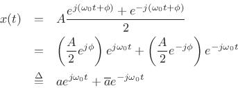
where
![]() denotes the complex conjugate of
denotes the complex conjugate of ![]() .
Thus, we can build a real sinusoid
.
Thus, we can build a real sinusoid ![]() as a linear combination of
positive- and negative-frequency complex sinusoidal components:
as a linear combination of
positive- and negative-frequency complex sinusoidal components:
where
 |
(6.3) |
The spectrum of ![]() is given by its
Fourier transform (see §2.2):
is given by its
Fourier transform (see §2.2):
![\begin{eqnarray*}
X(\omega) &\isdef & \int_{-\infty}^{\infty} x(t) e^{-j\omega t} dt\nonumber \\ [5pt]
&=& \int_{-\infty}^{\infty} \left[a s_{\omega_0}(t) + \overline{a} s_{-\omega_0}(t)
\right] e^{-j\omega t} dt.
\end{eqnarray*}](http://www.dsprelated.com/josimages_new/sasp2/img896.png)
In this case, ![]() is given by (5.2) and we have
is given by (5.2) and we have
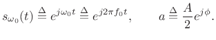
We see that, since the Fourier transform is a linear operator, we need only work with the unit-amplitude, zero-phase, positive-frequency sinusoid
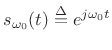 . For
. For
It remains to find the Fourier transform of
![]() :
:
![\begin{eqnarray*}
S_{\omega_0}(\omega)
&=& \int_{-\infty}^{\infty} s_{\omega_0}(t) e^{-j\omega t} dt\\ [5pt]
&\isdef & \int_{-\infty}^{\infty} e^{j\omega_0 t} e^{-j\omega t} dt\\ [5pt]
&=& \int_{-\infty}^{\infty} e^{j(\omega_0-\omega) t} dt\\ [5pt]
&=& \left.\frac{1}{j(\omega_0-\omega)} e^{j(\omega_0-\omega) t}
\right\vert _{-\infty}^\infty\\ [5pt]
&=& \lim_{\Delta\to\infty} 2\frac{\sin[(\omega_0-\omega)\Delta]}{\omega_0-\omega}\\ [5pt]
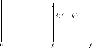
&=& 2\pi\delta(\omega_0-\omega) = \delta(f_0-f),
\end{eqnarray*}](http://www.dsprelated.com/josimages_new/sasp2/img902.png)
where
![]() is the delta function or impulse
at frequency
is the delta function or impulse
at frequency ![]() (see Fig.5.4 for a plot, and
§B.10 for a mathematical introduction).
Since the delta function is even (
(see Fig.5.4 for a plot, and
§B.10 for a mathematical introduction).
Since the delta function is even (
![]() ),
we can also write
),
we can also write
![]() . It is shown in §B.13 that the
sinc
limit
above approaches a delta function
. It is shown in §B.13 that the
sinc
limit
above approaches a delta function
![]() .
However, we will only use the Discrete Fourier Transform (DFT)
in any practical applications, and in that case, the result is easy to
show [264].
.
However, we will only use the Discrete Fourier Transform (DFT)
in any practical applications, and in that case, the result is easy to
show [264].
The inverse Fourier transform is easy to evaluate by the sifting property6.3of delta functions:
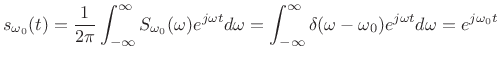 |
(6.6) |
Substituting into (5.4), the spectrum of our original sinusoid
![]() is given by
is given by
| (6.7) |
which is a pair of impulses, one at frequency
Spectrum of Sampled Complex Sinusoid
In the discrete-time case, we replace ![]() by
by ![]() where
where ![]() ranges
over the integers and
ranges
over the integers and ![]() is the sampling period in seconds. Thus,
for the positive-frequency component of the sinusoid of the previous
section, we obtain
is the sampling period in seconds. Thus,
for the positive-frequency component of the sinusoid of the previous
section, we obtain
 |
(6.8) |
It is common notational practice in signal processing to use normalized radian frequency
 |
(6.9) |
Thus, our sampled complex sinusoid becomes
 |
(6.10) |
It is not difficult to convert between normalized and unnormalized frequency. The use of a tilde (`
The spectrum of infinitely long discrete-time signals is given by the Discrete Time Fourier Transform (DTFT) (discussed in §2.1):
 |
(6.11) |
where now
Spectrum of a Windowed Sinusoid
Ideal sinusoids are infinite in duration. In practice, however, we must work with finite-length signals. Therefore, only a finite segment of a sinusoid can be processed at any one time, as if we were looking at the sinusoid through a ``window'' in time. For audio signals, the ear also processes sinusoids in short time windows (much less than 1 second long); thus, audio spectrum analysis is generally carried out using analysis windows comparable to the time-window inherent in hearing. Finally, nothing in nature produces true sinusoids. However, natural oscillations can often be modeled as sinusoidal over some finite time. Thus, it is useful to consider short-time spectrum analysis, in which the time-domain signal is analyzed in short time segments (windows). The short-time spectrum then evolves at some rate over time. The shorter our analysis window, the faster the short-time spectrum can change. Very long analysis windows, on the other hand, presuppose a fixed spectral content over the duration of the window.
The easiest windowing operation is simply truncating the sinusoid on the left and right at some finite times. This can be modeled mathematically as a multiplication of the sinusoid by the so-called rectangular window:
![$\displaystyle w_R(n) \isdef \left\{\begin{array}{ll} 1, & \left\vert n\right\vert\leq\frac{M-1}{2} \\ [5pt] 0, & \hbox{otherwise} \\ \end{array} \right.$](http://www.dsprelated.com/josimages_new/sasp2/img349.png) |
(6.12) |
where
 |
(6.13) |
![\includegraphics[width=4in]{eps/generalWindow}](http://www.dsprelated.com/josimages_new/sasp2/img925.png)
However, as we will see, it is often advantageous to taper the window more gracefully to zero on the left and right. Figure 5.1 illustrates the general shape of a more typical window function. Note that it is nonnegative and symmetric about time 0. Such functions are loosely called ``zero-phase'' since their Fourier transforms are real, as shown in §2.3. A more precise adjective is zero-centered for such windows.
In some cases, such as when analyzing real time systems, it is
appropriate to require our analysis windows be causal.
A window ![]() is said to be causal if it is zero for all
is said to be causal if it is zero for all ![]() .
Figure 5.2 depicts the causal version of the window shown in
Fig.5.1. A length
.
Figure 5.2 depicts the causal version of the window shown in
Fig.5.1. A length ![]() zero-centered
window can be made causal by shifting
(delaying) it in time by half its length
zero-centered
window can be made causal by shifting
(delaying) it in time by half its length ![]() . The shift theorem
(§2.3.4) tells us this introduces a linear phase term in
the frequency domain. That is, the window Fourier transform has gone
from being real to being multiplied by
. The shift theorem
(§2.3.4) tells us this introduces a linear phase term in
the frequency domain. That is, the window Fourier transform has gone
from being real to being multiplied by
![]() .
.
![\includegraphics[width=3.5in]{eps/causalWindow}](http://www.dsprelated.com/josimages_new/sasp2/img927.png)
Effect of Windowing
Let's look at a simple example of windowing to demonstrate what happens when we turn an infinite-duration signal into a finite-duration signal through windowing.
We begin with a sampled complex sinusoid:
| (6.14) |
A portion of the real part,
![\includegraphics[width=0.6\twidth]{eps/infDurSin}](http://www.dsprelated.com/josimages_new/sasp2/img931.png)
The Fourier transform of this infinite-duration signal is a delta
function at
![]() . I.e.,
. I.e.,
![]() , as indicated in Fig.5.4.
, as indicated in Fig.5.4.
The windowed signal is
| (6.15) |
as shown in Fig.5.5. (Note carefully the difference between
![\includegraphics[width=4in,height=2in]{eps/windowedSin}](http://www.dsprelated.com/josimages_new/sasp2/img934.png)
The convolution theorem (§2.3.5) tells
us that our multiplication in the time domain results in a convolution
in the frequency domain. Hence, we will obtain the convolution of
![]() with the Fourier transform of the window
with the Fourier transform of the window
![]() . This is easy since the delta function is the identity
element under convolution (
. This is easy since the delta function is the identity
element under convolution (
![]() ). However, since our
delta function is at frequency
). However, since our
delta function is at frequency
![]() , the
convolution shifts the window transform out to that frequency:
, the
convolution shifts the window transform out to that frequency:
| (6.16) |
This is shown in Fig.5.6.
![\includegraphics[width=\twidth]{eps/windowedSinSpec}](http://www.dsprelated.com/josimages_new/sasp2/img938.png) |
From comparing Fig.5.6 with the ideal sinusoidal
spectrum in Fig.5.4 (an impulse at frequency ![]() ),
we can make some observations:
),
we can make some observations:
- Windowing in the time domain resulted in a ``smearing''
or ``smoothing'' in the frequency domain. In particular, the
infinitely thin delta function has been replaced by the ``main lobe''
of the window transform. We need to be aware of this if we are trying
to resolve sinusoids which are close together in frequency.
- Windowing also introduced side lobes. This is important
when we are trying to resolve low amplitude sinusoids in the presence
of higher amplitude signals.
- A sinusoid at amplitude
 , frequency
  , and phase
 manifests (in practical spectrum analysis) as a
window transform shifted out to frequency
, and scaled
by
manifests (in practical spectrum analysis) as a
window transform shifted out to frequency
, and scaled
by
 .
.
As a result of the last point above, the ideal window transform is an impulse in the frequency domain. Since this cannot be achieved in practice, we try to find spectrum-analysis windows which approximate this ideal in some optimal sense. In particular, we want side-lobes that are as close to zero as possible, and we want the main lobe to be as tall and narrow as possible. (Since absolute scalings are normally arbitrary in signal processing, ``tall'' can be defined as the ratio of main-lobe amplitude to side-lobe amplitude--or main-lobe energy to side-lobe energy, etc.) There are many alternative formulations for ``approximating an impulse'', and each such formulation leads to a particular spectrum-analysis window which is optimal in that sense. In addition to these windows, there are many more which arise in other applications. Many commonly used window types are summarized in Chapter 3.
Frequency Resolution
The frequency resolution of a spectrum-analysis window is determined by its main-lobe width (Chapter 3) in the frequency domain, where a typical main lobe is illustrated in Fig.5.6 (top). For maximum frequency resolution, we desire the narrowest possible main-lobe width, which calls for the rectangular window (§3.1), the transform of which is shown in Fig.3.3. When we cannot be fooled by the large side-lobes of the rectangular window transform (e.g., when the sinusoids under analysis are known to be well separated in frequency), the rectangular window truly is the optimal window for the estimation of frequency, amplitude, and phase of a sinusoid in the presence of stationary noise [230,120,121].
The rectangular window has only one parameter (aside from amplitude)--its length. The next section looks at the effect of an increased window length on our ability to resolve two sinusoids.
Two Cosines (``In-Phase'' Case)
Figure 5.7 shows a spectrum analysis of two cosines
| (6.17) |
where
 ).
The length
).
The length
![\includegraphics[width=\twidth]{eps/resolvedSines}](http://www.dsprelated.com/josimages_new/sasp2/img951.png)
The longest window (![]() ) resolves the sinusoids very well, while
the shortest case (
) resolves the sinusoids very well, while
the shortest case (![]() ) does not resolve them at all (only one
``lump'' appears in the spectrum analysis). In difference-frequency
cycles, the analysis windows are two cycles and half a cycle in these
cases, respectively. It can be debated whether or not the other two
cases are resolved, and we will return to them shortly.
) does not resolve them at all (only one
``lump'' appears in the spectrum analysis). In difference-frequency
cycles, the analysis windows are two cycles and half a cycle in these
cases, respectively. It can be debated whether or not the other two
cases are resolved, and we will return to them shortly.
One Sine and One Cosine ``Phase Quadrature'' Case
Figure 5.8 shows a similar spectrum analysis of two sinusoids
| (6.18) |
using the same frequency separation and window lengths. However, now the sinusoids are 90 degrees out of phase (one sine and one cosine). Curiously, the top-left case (
![\includegraphics[width=\twidth]{eps/resolvedSinesB}](http://www.dsprelated.com/josimages_new/sasp2/img956.png)
Figure 5.9 shows the same plots as in Fig.5.8, but overlaid. From this we can see that the peak locations are biased in under-resolved cases, both in amplitude and frequency.
![\includegraphics[width=\textwidth ]{eps/resolvedSinesC2C}](http://www.dsprelated.com/josimages_new/sasp2/img957.png)
The preceding figures suggest that, for a rectangular window of length
![]() , two sinusoids are well resolved when they are separated in
frequency by
, two sinusoids are well resolved when they are separated in
frequency by
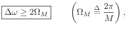 |
(6.19) |
where the frequency-separation
 |
(6.20) |
where the
 denotes normalized frequency in
cycles per sample. In Hz, we have
denotes normalized frequency in
cycles per sample. In Hz, we have
 |
(6.21) |
or
 |
(6.22) |
Note that
A more detailed study [1] reveals that ![]() cycles
of the difference-frequency is sufficient to enable fully accurate
peak-frequency measurement under the rectangular window by means of
finding FFT peaks. In §5.5.2 below, additional minimum duration
specifications for resolving closely spaced sinusoids are given for
other window types as well.
cycles
of the difference-frequency is sufficient to enable fully accurate
peak-frequency measurement under the rectangular window by means of
finding FFT peaks. In §5.5.2 below, additional minimum duration
specifications for resolving closely spaced sinusoids are given for
other window types as well.
In principle, we can resolve arbitrarily small frequency separations, provided
- there is no noise, and
- we are sure we are looking at the sum of two ideal sinusoids under the window.
The rectangular window provides an abrupt transition at its edge. While it remains the optimal window for sinusoidal peak estimation, it is by no means optimal in all spectrum analysis and/or signal processing applications involving spectral processing. As discussed in Chapter 3, windows with a more gradual transition to zero have lower side-lobe levels, and this is beneficial for spectral displays and various signal processing applications based on FFT methods. We will encounter such applications in later chapters.
Resolving Sinusoids
We saw in §5.4.1 that our ability to resolve two closely spaced sinusoids is determined by the main-lobe width of the window transform we are using. We will now study this relationship in more detail.
For starters, let's define main-lobe bandwidth very simply (and
somewhat crudely) as the distance between the first
zero-crossings on either side of the main lobe, as shown in
Fig.5.10 for a rectangular-window transform. Let ![]() denote this width in Hz. In normalized radian frequency units, as
used in the frequency axis of Fig.5.10,
denote this width in Hz. In normalized radian frequency units, as
used in the frequency axis of Fig.5.10, ![]() Hz translates to
Hz translates to
![]() radians per sample, where
radians per sample, where ![]() denotes the sampling rate in Hz.
denotes the sampling rate in Hz.
![\includegraphics[width=\twidth]{eps/rectWinMLM}](http://www.dsprelated.com/josimages_new/sasp2/img967.png)
For the length-![]() unit-amplitude rectangular window defined in
§3.1, the DTFT is given analytically by
unit-amplitude rectangular window defined in
§3.1, the DTFT is given analytically by
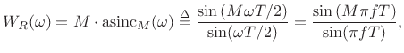
where
 |
(6.24) |
as can be seen in Fig.5.10.
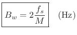
Recall from §3.1.1 that the side-lobe width in a
rectangular-window transform (![]() Hz) is given in radians
per sample by
Hz) is given in radians
per sample by
 |
(6.25) |
As Fig.5.10 illustrates, the rectangular-window transform main-lobe width is
|
Other Definitions of Main Lobe Width
Our simple definition of main-lobe band-width (distance between zero-crossings) works pretty well for windows in the Blackman-Harris family, which includes the first six entries in Table 5.1. (See §3.3 for more about the Blackman-Harris window family.) However, some windows have smooth transforms, such as the Hann-Poisson (Fig.3.21), or infinite-duration Gaussian window (§3.11). In particular, the true Gaussian window has a Gaussian Fourier transform, and therefore no zero crossings at all in either the time or frequency domains. In such cases, the main-lobe width is often defined using the second central moment.6.5
A practical engineering definition of main-lobe width is the minimum distance about the center such that the window-transform magnitude does not exceed the specified side-lobe level anywhere outside this interval. Such a definition always gives a smaller main-lobe width than does a definition based on zero crossings.
![\includegraphics[width=3in]{eps/windowParameters}](http://www.dsprelated.com/josimages_new/sasp2/img976.png)
In filter-design terminology, regarding the window as an FIR filter and its transform as a lowpass-filter frequency response [263], as depicted in Fig.5.11, we can say that the side lobes are everything in the stop band, while the main lobe is everything in the pass band plus the transition band of the frequency response. The pass band may be defined as some small interval about the midpoint of the main lobe. The wider the interval chosen, the larger the ``ripple'' in the pass band. The pass band can even be regarded as having zero width, in which case the main lobe consists entirely of transition band. This formulation is quite useful when designing customized windows by means of FIR filter design software, such as in Matlab or Octave (see §4.5.1, §4.10, and §3.13).
Simple Sufficient Condition for Peak Resolution
Recall from §5.4 that the frequency-domain image of a
sinusoid ``through a window'' is the window transform scaled by the
sinusoid's amplitude and shifted so that the main lobe is centered
about the sinusoid's frequency. A spectrum analysis of two sinusoids
summed together is therefore, by linearity of the Fourier transform,
the sum of two overlapping window transforms, as shown in
Fig.5.12 for the rectangular window. A simple
sufficient requirement for resolving two sinusoidal
peaks spaced ![]() Hz apart is to choose a window length long
enough so that the main lobes are clearly separated when the
sinusoidal frequencies are separated by
Hz apart is to choose a window length long
enough so that the main lobes are clearly separated when the
sinusoidal frequencies are separated by ![]() Hz. For example, we
may require that the main lobes of any Blackman-Harris window meet at
the first zero crossings in the worst case (narrowest frequency
separation); this is shown in Fig.5.12 for the rectangular-window.
Hz. For example, we
may require that the main lobes of any Blackman-Harris window meet at
the first zero crossings in the worst case (narrowest frequency
separation); this is shown in Fig.5.12 for the rectangular-window.
![\includegraphics[width=\twidth]{eps/sinesAnn}](http://www.dsprelated.com/josimages_new/sasp2/img978.png)
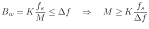
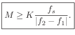
To obtain the separation shown in Fig.5.12, we must have
![]() Hz, where
Hz, where ![]() is the main-lobe width in Hz, and
is the main-lobe width in Hz, and
![]() is the minimum sinusoidal frequency separation in Hz.
is the minimum sinusoidal frequency separation in Hz.
For members of the ![]() -term Blackman-Harris window family,
-term Blackman-Harris window family, ![]() can
be expressed as
can
be expressed as
![]() , as indicated by
Table 5.1. In normalized radian frequency units, i.e.,
radians per sample, we have
, as indicated by
Table 5.1. In normalized radian frequency units, i.e.,
radians per sample, we have
![]() . For comparison, Table 5.2 lists minimum effective
values of
. For comparison, Table 5.2 lists minimum effective
values of ![]() for each window (denoted
for each window (denoted ![]() ) given by an
empirically verified sharper lower bound on the value needed for
accurate peak-frequency measurement [1], as discussed
further in §5.5.4 below.
) given by an
empirically verified sharper lower bound on the value needed for
accurate peak-frequency measurement [1], as discussed
further in §5.5.4 below.
|
We make the main-lobe width ![]() smaller by increasing the window
length
smaller by increasing the window
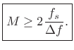
length ![]() . Specifically, requiring
. Specifically, requiring
![]() Hz implies
Hz implies
 |
(6.26) |
or
Thus, to resolve the frequencies
Periodic Signals
Many signals are periodic in nature, such as short segments of
most tonal musical instruments and speech. The sinusoidal components
in a periodic signal are constrained to be harmonic, that is,
occurring at frequencies that are an integer multiple of the
fundamental frequency ![]() .6.6 Physically, any ``driven
oscillator,'' such as bowed-string instruments, brasses, woodwinds,
flutes, etc., is usually quite periodic in normal steady-state
operation, and therefore generates harmonic overtones in steady
state. Freely vibrating resonators, on the other hand, such as
plucked strings, gongs, and ``tonal percussion'' instruments,
are not generally periodic.6.7
.6.6 Physically, any ``driven
oscillator,'' such as bowed-string instruments, brasses, woodwinds,
flutes, etc., is usually quite periodic in normal steady-state
operation, and therefore generates harmonic overtones in steady
state. Freely vibrating resonators, on the other hand, such as
plucked strings, gongs, and ``tonal percussion'' instruments,
are not generally periodic.6.7
Consider a periodic signal with fundamental frequency ![]() Hz.
Then the harmonic components occur at integer multiples of
Hz.
Then the harmonic components occur at integer multiples of ![]() , and
so they are spaced in frequency by
, and
so they are spaced in frequency by
![]() . To resolve
these harmonics in a spectrum analysis, we require, adapting
(5.27),
. To resolve
these harmonics in a spectrum analysis, we require, adapting
(5.27),
 |
(6.28) |
Note that
 is the fundamental period of the signal in samples.
Thus, another way of stating our simple, sufficient resolution
requirement on window length
is the fundamental period of the signal in samples.
Thus, another way of stating our simple, sufficient resolution
requirement on window length
Specifically, resolving the harmonics of a periodic signal with period
![]() samples is assured if we have at least
samples is assured if we have at least
 periods under the rectangular window,
 periods under the Hamming window,
 periods under the Blackman window,
 periods under the Blackman-Harris
  -term window,
![\begin{figure*}\centering
\subfigure[Length $M=100$\ rectangular window]{
\epsfxsize =\twidth
\epsfysize =1.5in \epsfbox{eps/EffectiveLength1.eps}
}
\subfigure[Length $M=200$\ Hamming window]{
\epsfxsize =\twidth
\epsfysize =1.5in \epsfbox{eps/EffectiveLength2.eps}
}
\subfigure[Length $M=300$\ Blackman window]{
\epsfxsize =\twidth
\epsfysize =1.5in \epsfbox{eps/EffectiveLength3.eps}
}\end{figure*}](http://www.dsprelated.com/josimages_new/sasp2/img1005.png) |
Tighter Bounds for Minimum Window Length
[This section, adapted from [1], is relatively advanced and may be skipped without loss of continuity.]
Figures 5.14(a) through 5.14(d) show four possible definitions of main-lobe separation that could be considered for purposes of resolving closely spaced sinusoidal peaks.
![\begin{figure*}\centering
\subfigure[Minimum orthogonal separation]{
\epsfxsize =4.0in
\epsfysize =1.0in \epsfbox{eps/SpecResCases1.eps}
}
\subfigure[Separation to first stationary-point \cite{AbeAndSmith04}]{
\epsfxsize =4.0in
\epsfysize =1.0in \epsfbox{eps/SpecResCases2.eps}
}
\subfigure[Separation to where main-lobe level equals side-lobe level]{
\epsfxsize =4.0in
\epsfysize =1.0in \epsfbox{eps/SpecResCases3.eps}
}
\subfigure[Full main-lobe separation]{
\epsfxsize =4.0in
\epsfysize =1.0in \epsfbox{eps/SpecResCases4.eps}
}\end{figure*}](http://www.dsprelated.com/josimages_new/sasp2/img1006.png) |
In Fig.5.14(a), the main lobes sit atop each other's first zero
crossing. We may call this the ``minimum orthogonal separation,'' so
named because we know from Discrete Fourier Transform theory
[264] that ![]() -sample segments of sinusoids at this
frequency-spacing are exactly orthogonal. (
-sample segments of sinusoids at this
frequency-spacing are exactly orthogonal. (![]() is the
rectangular-window length as before.) At this spacing, the peak of
each main lobe is unchanged by the ``interfering'' window transform.
However, the slope and higher derivatives at each peak
are modified by the presence of the interfering window
transform. In practice, we must work over a discrete frequency axis,
and we do not, in general, sample exactly at each main-lobe peak.
Instead, we usually determine an interpolated peak location
based on samples near the true peak location. For example, quadratic
interpolation, which is commonly used, requires at least three samples
about each peak (as discussed in §5.7 below), and it is
therefore sensitive to a nonzero slope at the peak. Thus, while
minimum-orthogonal spacing is ideal in the limit as the sampling
density along the frequency axis approaches infinity, it is not ideal
in practice, even when we know the peak frequency-spacing
exactly.6.8
is the
rectangular-window length as before.) At this spacing, the peak of
each main lobe is unchanged by the ``interfering'' window transform.
However, the slope and higher derivatives at each peak
are modified by the presence of the interfering window
transform. In practice, we must work over a discrete frequency axis,
and we do not, in general, sample exactly at each main-lobe peak.
Instead, we usually determine an interpolated peak location
based on samples near the true peak location. For example, quadratic
interpolation, which is commonly used, requires at least three samples
about each peak (as discussed in §5.7 below), and it is
therefore sensitive to a nonzero slope at the peak. Thus, while
minimum-orthogonal spacing is ideal in the limit as the sampling
density along the frequency axis approaches infinity, it is not ideal
in practice, even when we know the peak frequency-spacing
exactly.6.8
Figure 5.14(b) shows the ``zero-error stationary point'' frequency
spacing. In this case, the main-lobe peak of one
![]() sits atop
the first local minimum from the main-lobe of the other
sits atop
the first local minimum from the main-lobe of the other
![]() . Since the derivative of both
. Since the derivative of both
![]() functions is zero at
both peak frequencies at this spacing, the peaks do not ``sit on a
slope'' which would cause the peak locations to be biased away
from the sinusoidal frequencies. We may say that peak-frequency
estimates based on samples about the peak will be unbiased, to first
order, at this spacing. This minimum spacing, which is easy to
compute for Blackman-Harris windows, turns out to be very close to the
optimal minimum spacing [1].
functions is zero at
both peak frequencies at this spacing, the peaks do not ``sit on a
slope'' which would cause the peak locations to be biased away
from the sinusoidal frequencies. We may say that peak-frequency
estimates based on samples about the peak will be unbiased, to first
order, at this spacing. This minimum spacing, which is easy to
compute for Blackman-Harris windows, turns out to be very close to the
optimal minimum spacing [1].
Figure 5.14(c) shows the minimum frequency spacing which naturally matches side-lobe level. That is, the main lobes are pulled apart until the main-lobe level equals the worst-case side-lobe level. This spacing is usually not easy to compute, and it is best matched with the Chebyshev window (see §3.10). Note that it is just a little wider than the stationary-point spacing discussed in the previous paragraph.
For ease of comparison, Fig.5.14(d) shows once again the simple, sufficient rule (''full main-lobe separation'') discussed in §5.5.2 above. While overly conservative, it is easily computed for many window types (any window with a known main-lobe width), and so it remains a useful rule-of-thumb for determining minimum window length given the minimum expected frequency spacing.
A table of minimum window lengths for the Kaiser window, as a function of frequency spacing, is given in §3.9.
Summary
We see that when measuring sinusoidal peaks, it is important to know the minimum frequency separation of the peaks, and to choose an FFT window which is long enough to resolve the peaks accurately. Generally speaking, the window must ``see'' at least 1.5 cycles of the minimum difference frequency. The rectangular window ``sees'' its full length. Other windows, which are all tapered in some way (Chapter 3), see an effective duration less than the window length in samples. Further details regarding theoretical and empirical estimates are given in [1].
Sinusoidal Peak Interpolation
In §2.5, we discussed ideal spectral interpolation (zero-padding in the time domain followed by an FFT). Since FFTs are efficient, this is an efficient interpolation method. However, in audio spectral modeling, there is usually a limit on the needed accuracy due to the limitations of audio perception. As a result, a ``perceptually ideal'' spectral interpolation method that is even more efficient is to zero-pad by some small factor (usually less than 5), followed by quadratic interpolation of the spectral magnitude. We call this the quadratically interpolated FFT (QIFFT) method [271,1]. The QIFFT method is usually more efficient than the equivalent degree of ideal interpolation, for a given level of perceptual error tolerance (specific guidelines are given in §5.6.2 below). The QIFFT method can be considered an approximate maximum likelihood method for spectral peak estimation, as we will see.
Quadratic Interpolation of Spectral Peaks
In quadratic interpolation of sinusoidal spectrum-analysis peaks, we replace the main lobe of our window transform by a quadratic polynomial, or ``parabola''. This is valid for any practical window transform in a sufficiently small neighborhood about the peak, because the higher order terms in a Taylor series expansion about the peak converge to zero as the peak is approached.
Note that, as mentioned in §D.1, the Gaussian window transform magnitude is precisely a parabola on a dB scale. As a result, quadratic spectral peak interpolation is exact under the Gaussian window. Of course, we must somehow remove the infinitely long tails of the Gaussian window in practice, but this does not cause much deviation from a parabola, as shown in Fig.3.36.
![\begin{psfrags}
% latex2html id marker 16827\psfrag{a} []{ \Large$ \alpha $}\psfrag{b} []{ \Large$ \beta $}\psfrag{g} []{ \Large$ \gamma $\ }\begin{figure}[htbp]
\includegraphics[width=\textwidth ]{eps/parabola}
\caption{Illustration of
parabolic peak interpolation using the three samples nearest the peak.}
\end{figure}
\end{psfrags}](http://www.dsprelated.com/josimages_new/sasp2/img1007.png)
Referring to Fig.5.15, the general formula for a parabola may be written as
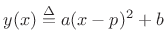 |
(6.29) |
The center point
At the three samples nearest the peak, we have
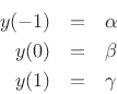
where we arbitrarily renumbered the bins about the peak ![]() , 0, and 1.
Writing the three samples in terms of the interpolating parabola gives
, 0, and 1.
Writing the three samples in terms of the interpolating parabola gives
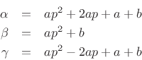
which implies
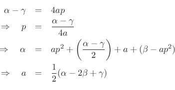
Hence, the interpolated peak location is given in bins6.9 (spectral samples) by
![$\displaystyle \zbox {p=\frac{1}{2}\frac{\alpha-\gamma}{\alpha-2\beta+\gamma}} \in [-1/2,1/2].$](http://www.dsprelated.com/josimages_new/sasp2/img1015.png) |
(6.30) |
If
Using the interpolated peak location, the peak magnitude estimate is
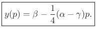 |
(6.31) |
Phase Interpolation at a Peak
Note that only the spectral magnitude is used to find ![]() in
the parabolic interpolation scheme of the previous section. In some
applications, a phase interpolation is also desired.
in
the parabolic interpolation scheme of the previous section. In some
applications, a phase interpolation is also desired.
In principle, phase interpolation is independent of magnitude interpolation, and any interpolation method can be used. There is usually no reason to expect a ``phase peak'' at a magnitude peak, so simple linear interpolation may be used to interpolate the unwrapped phase samples (given a sufficiently large zero-padding factor). Matlab has an unwrap function for unwrapping phase, and §F.4 provides an Octave-compatible version.
If we do expect a phase peak (such as when identifying chirps, as discussed in §10.6), then we may use quadratic interpolation separately on the (unwrapped) phase.
Alternatively, the real and imaginary parts can be interpolated separately to yield a complex peak value estimate.
Matlab for Parabolic Peak Interpolation
Section §F.2 lists Matlab/Octave code for finding quadratically interpolated peaks in the magnitude spectrum as discussed above. At the heart is the qint function, which contains the following:
function [p,y,a] = qint(ym1,y0,yp1)
%QINT - quadratic interpolation of three adjacent samples
%
% [p,y,a] = qint(ym1,y0,yp1)
%
% returns the extremum location p, height y, and half-curvature a
% of a parabolic fit through three points.
% Parabola is given by y(x) = a*(x-p)^2+b,
% where y(-1)=ym1, y(0)=y0, y(1)=yp1.

p = (yp1 - ym1)/(2*(2*y0 - yp1 - ym1));
y = y0 - 0.25*(ym1-yp1)*p;
a = 0.5*(ym1 - 2*y0 + yp1);
Bias of Parabolic Peak Interpolation
Since the true window transform is not a parabola (except for the conceptual case of a Gaussian window transform expressed in dB), there is generally some error in the interpolated peak due to this mismatch. Such a systematic error in an estimated quantity (due to modeling error, not noise), is often called a bias. Parabolic interpolation is unbiased when the peak occurs at a spectral sample (FFT bin frequency), and also when the peak is exactly half-way between spectral samples (due to symmetry of the window transform about its midpoint). For other peak frequencies, quadratic interpolation yields a biased estimate of both peak frequency and peak amplitude. (Phase is essentially unbiased [1].)
Since zero-padding in the time domain gives ideal interpolation in the frequency domain, there is no bias introduced by this type of interpolation. Thus, if enough zero-padding is used so that a spectral sample appears at the peak frequency, simply finding the largest-magnitude spectral sample will give an unbiased peak-frequency estimator. (We will learn in §5.7.2 that this is also the maximum likelihood estimator for the frequency of a sinusoid in additive white Gaussian noise.)
While we could choose our zero-padding factor large enough to yield any desired degree of accuracy in peak frequency measurements, it is more efficient in practice to combine zero-padding with parabolic interpolation (or some other simple, low-order interpolator). In such hybrid schemes, the zero-padding is simply chosen large enough so that the bias due to parabolic interpolation is negligible. In §5.7 below, the Quadratically Interpolated FFT (QIFFT) method is described as one such hybrid scheme.
Optimal Peak-Finding in the Spectrum
Based on the preceding sections, an ``obvious'' method for deducing sinusoidal parameters from data is to find the amplitude, phase, and frequency of each peak in a zero-padded FFT of the data. We have considered so far the following issues:
- Make sure the data length (or window length) is long enough so that all sinusoids in the data are resolved.
- Use enough zero padding so that the spectrum is heavily oversampled, making the peaks easier to interpolate.
- Use quadratic interpolation of the three samples surrounding a dB-magnitude peak in the heavily oversampled spectrum.
- Evaluate the fitted parabola at its extremum to obtain the interpolated amplitude and frequency estimates for each sinusoidal component.
- Similarly compute a phase estimate at each peak frequency using quadratic or even linear interpolation on the unwrapped phase samples about the peak.
The question naturally arises as to how good is the QIFFT method for spectral peak estimation? Is it optimal in any sense? Are there better methods? Are there faster methods that are almost as good? These are questions that generally fall under the topic of sinusoidal parameter estimation.
We will show that the QIFFT method is a fast, ``approximate maximum-likelihood method.'' When properly configured, it is in fact extremely close to the true maximum-likelihood estimator for a single sinusoid in white noise. It is also close to the maximum likelihood estimator for multiple sinusoids that are well separated in frequency (i.e., side-lobe overlap can be neglected). Finally, the QIFFT method can be considered optimal perceptually in the sense that any errors induced by the suboptimality of the QIFFT method are inaudible when the zero-padding factor is a factor of 5 or more. While a zero-padding factor of 5 is sufficient for all window types, including the rectangular window, less zero-padding is needed with windows having flatter main-lobe peaks, as summarized in Table 5.3.
Minimum Zero-Padding for High-Frequency Peaks
|
Table 5.3 gives zero-padding factors sufficient for keeping
the bias below
![]() Hz, where
Hz, where ![]() denotes the sampling
rate in Hz, and
denotes the sampling
rate in Hz, and ![]() is the window length in samples. For fundamental
frequency estimation,
is the window length in samples. For fundamental
frequency estimation, ![]() can be interpreted as the
relative frequency error ``
can be interpreted as the
relative frequency error ``
![]() '' when the window
length is one period. In this case,
'' when the window
length is one period. In this case, ![]() is the fundamental
frequency in Hz. More generally,
is the fundamental
frequency in Hz. More generally, ![]() is the bandwidth of each
side-lobe in the DTFT of a length
is the bandwidth of each
side-lobe in the DTFT of a length ![]() rectangular, generalized
Hamming, or Blackman window (any member of the Blackman-Harris window
family, as elaborated in Chapter 3).
rectangular, generalized
Hamming, or Blackman window (any member of the Blackman-Harris window
family, as elaborated in Chapter 3).
Note from Table 5.3 that the Blackman window requires no
zero-padding at all when only ![]() % accuracy is required in
peak-frequency measurement. It should also be understood that a
frequency error of
% accuracy is required in
peak-frequency measurement. It should also be understood that a
frequency error of ![]() % is inaudible in most audio
applications.6.10
% is inaudible in most audio
applications.6.10
Minimum Zero-Padding for Low-Frequency Peaks
Sharper bounds on the zero-padding factor needed for low-frequency
peaks (below roughly 1 kHz) may be obtained based on the measured
Just-Noticeable-Difference (JND) in frequency and/or amplitude
[276]. In particular, a ![]() % relative-error
spec is good above 1 kHz (being conservative by approximately a factor
of 2), but overly conservative at lower frequencies where the JND
flattens out. Below 1 kHz, a fixed 1 Hz spec satisfies perceptual
requirements and gives smaller minimum zero-padding factors than the
% relative-error
spec is good above 1 kHz (being conservative by approximately a factor
of 2), but overly conservative at lower frequencies where the JND
flattens out. Below 1 kHz, a fixed 1 Hz spec satisfies perceptual
requirements and gives smaller minimum zero-padding factors than the
![]() % relative-error spec.
% relative-error spec.
The following data, extracted from [276, Table I, p. 89] gives frequency JNDs at a presentation level of 60 dB SPL (the most sensitive case measured):
  f =    [    62,    125,    250,    500,   1000,   2000,   4000];
  dfof = [0.0346, 0.0269, 0.0098, 0.0035, 0.0034, 0.0018, 0.0020];
Thus, the frequency JND at 4 kHz was measured to be two tenths of a percent. (These measurements were made by averaging experimental results for five men between the ages of 20 and 30.) Converting relative frequency to absolute frequency in Hz yields (in matlab syntax):
df = dfof .* f; % = [2.15, 3.36, 2.45, 1.75, 3.40, 3.60, 8.00];For purposes of computing the minimum zero-padding factor required, we see that the absolute tuning error due to bias can be limited to 1 Hz, based on measurements at 500 Hz (at 60 dB). Doing this for frequencies below 1 kHz yields the results shown in Table 5.4. Note that the Blackman window needs no zero padding below 125 Hz, and the Hamming/Hann window requires no zero padding below 62.5 Hz.
|
Matlab for Computing Minimum Zero-Padding Factors
The minimum zero-padding factors in the previous two subsections were computed using the matlab function zpfmin listed in §F.2.4. For example, both tables above are included in the output of the following matlab program:
  windows={'rect','hann','hamming','blackman'};
  freqs=[1000,500,250,125,62.5];
  for i=1:length(windows)
    w = sprintf("%s",windows(i))
    for j=1:length(freqs)
      f = freqs(j);
      zpfmin(w,1/f,0.01*f)  % 1 percent spec (large for audio)
      zpfmin(w,1/f,0.001*f) % 0.1 percent spec (good > 1 kHz)
      zpfmin(w,1/f,1)       % 1 Hz spec (good below 1 kHz)
    end
  end
In addition to ``perceptually exact'' detection of spectral peaks, there are times when we need to find spectral parameters as accurately as possible, irrespective of perception. For example, one can estimate the stiffness of a piano string by measuring the stretched overtone-frequencies in the spectrum of that string's vibration. Additionally, we may have measurement noise, in which case we want our measurements to be minimally influenced by this noise. The following sections discuss optimal estimation of spectral-peak parameters due to sinusoids in the presence of noise.
Least Squares Sinusoidal Parameter Estimation
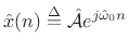
There are many ways to define ``optimal'' in signal modeling. Perhaps the most elementary case is least squares estimation. Every estimator tries to measure one or more parameters of some underlying signal model. In the case of sinusoidal parameter estimation, the simplest model consists of a single complex sinusoidal component in additive white noise:
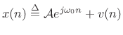
where
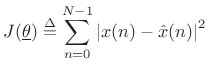
with respect to the parameter vector
![$\displaystyle \underline{\theta}\isdef \left[\begin{array}{c} A \\ [2pt] \phi \\ [2pt] \omega_0 \end{array}\right],$](http://www.dsprelated.com/josimages_new/sasp2/img1033.png) |
(6.34) |
where
 |
(6.35) |
Note that the error signal
Sinusoidal Amplitude Estimation
If the sinusoidal frequency ![]() and phase
and phase ![]() happen to be
known, we obtain a simple linear least squares problem for the
amplitude
happen to be
known, we obtain a simple linear least squares problem for the
amplitude ![]() . That is, the error signal
. That is, the error signal
| (6.36) |
becomes linear in the unknown parameter
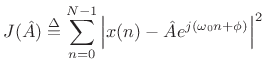
becomes a simple quadratic (parabola) over the real line.6.11 Quadratic forms in any number of dimensions are easy to minimize. For example, the ``bottom of the bowl'' can be reached in one step of Newton's method. From another point of view, the optimal parameter
Yet a third way to minimize (5.37) is the method taught in
elementary calculus: differentiate
![]() with respect to
with respect to ![]() , equate
it to zero, and solve for
, equate
it to zero, and solve for ![]() . In preparation for this, it is helpful to
write (5.37) as
. In preparation for this, it is helpful to
write (5.37) as
![\begin{eqnarray*}
J({\hat A}) &\isdef & \sum_{n=0}^{N-1}
\left[x(n)-{\hat A}e^{j(\omega_0 n+\phi)}\right]
\left[\overline{x(n)}-\overline{{\hat A}} e^{-j(\omega_0 n+\phi)}\right]\\
&=&
\sum_{n=0}^{N-1}
\left[
\left\vert x(n)\right\vert^2
-
x(n)\overline{{\hat A}} e^{-j(\omega_0 n+\phi)}
-
\overline{x(n)}{\hat A}e^{j(\omega_0 n+\phi)}
+
{\hat A}^2
\right]
\\
&=& \left\Vert\,x\,\right\Vert _2^2 - 2\mbox{re}\left\{\sum_{n=0}^{N-1} x(n)\overline{{\hat A}}
e^{-j(\omega_0 n+\phi)}\right\}
+ N {\hat A}^2.
\end{eqnarray*}](http://www.dsprelated.com/josimages_new/sasp2/img1045.png)
Differentiating with respect to ![]() and equating to zero yields
and equating to zero yields
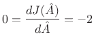 re re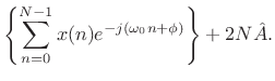 |
(6.38) |
Solving this for
 re
re re
reThat is, the optimal least-squares amplitude estimate may be found by the following steps:
- Multiply the data
 by
by
 to zero the known phase
.
to zero the known phase
.
- Take the DFT of the
 samples of
  , suitably zero padded to approximate the DTFT, and evaluate it at the known frequency
.
, suitably zero padded to approximate the DTFT, and evaluate it at the known frequency
.
- Discard any imaginary part since it can only contain noise, by (5.39).
- Divide by
to obtain a properly normalized coefficient of projection
[264] onto the sinusoid
(6.40)
Sinusoidal Amplitude and Phase Estimation
The form of the optimal estimator (5.39) immediately suggests the following generalization for the case of unknown amplitude and phase:
That is,
The orthogonality principle for linear least squares estimation states
that the projection error must be orthogonal to the model.
That is, if ![]() is our optimal signal model (viewed now as an
is our optimal signal model (viewed now as an
![]() -vector in
-vector in ![]() ), then we must have [264]
), then we must have [264]

Thus, the complex coefficient of projection of ![]() onto
onto
![]() is given by
is given by
 |
(6.42) |
The optimality of
 |
Sinusoidal Frequency Estimation
The form of the least-squares estimator (5.41) in the known-frequency case immediately suggests the following frequency estimator for the unknown-frequency case:
That is, the sinusoidal frequency estimate is defined as that frequency which maximizes the DTFT magnitude. Given this frequency, the least-squares sinusoidal amplitude and phase estimates are given by (5.41) evaluated at that frequency.
It can be shown [121] that (5.43) is in fact the optimal least-squares estimator for a single sinusoid in white noise. It is also the maximum likelihood estimator for a single sinusoid in Gaussian white noise, as discussed in the next section.
In summary,
In practice, of course, the DTFT is implemented as an interpolated FFT, as described in the previous sections (e.g., QIFFT method).
Maximum Likelihood Sinusoid Estimation
The maximum likelihood estimator (MLE) is widely used in practical signal modeling [121]. A full treatment of maximum likelihood estimators (and statistical estimators in general) lies beyond the scope of this book. However, we will show that the MLE is equivalent to the least squares estimator for a wide class of problems, including well resolved sinusoids in white noise.
Consider again the signal model of (5.32) consisting of a complex sinusoid in additive white (complex) noise:
Again,
 |
(6.46) |
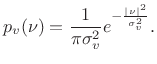
We express the zero-mean Gaussian assumption by writing
| (6.47) |
The parameter
It turns out that when Gaussian random variables ![]() are
uncorrelated (i.e., when
are
uncorrelated (i.e., when ![]() is white noise), they are also
independent. This means that the probability of observing
particular values of
is white noise), they are also
independent. This means that the probability of observing
particular values of ![]() and
and ![]() is given by the product of
their respective probabilities [121]. We will now use this
fact to compute an explicit probability for observing any data
sequence
is given by the product of
their respective probabilities [121]. We will now use this
fact to compute an explicit probability for observing any data
sequence ![]() in (5.44).
in (5.44).
Since the sinusoidal part of our signal model,
![]() , is deterministic; i.e., it does not including any random
components; it may be treated as the time-varying mean of a
Gaussian random process
, is deterministic; i.e., it does not including any random
components; it may be treated as the time-varying mean of a
Gaussian random process ![]() . That is, our signal model
(5.44) can be rewritten as
. That is, our signal model
(5.44) can be rewritten as
| (6.48) |
and the probability density function for the whole set of observations
![$\displaystyle p(x) = p[x(0)] p[x(1)]\cdots p[x(N-1)] = \left(\frac{1}{\pi \sigma_v^2}\right)^N e^{-\frac{1}{\sigma_v^2}\sum_{n=0}^{N-1} \left\vert x(n) - {\cal A}e^{j\omega_0 n}\right\vert^2}$](http://www.dsprelated.com/josimages_new/sasp2/img1079.png) |
(6.49) |
Thus, given the noise variance
Likelihood Function
The likelihood function
![]() is defined as the
probability density function of
is defined as the
probability density function of ![]() given
given
![]() , evaluated at a particular
, evaluated at a particular ![]() , with
, with
![]() regarded as a variable.
regarded as a variable.
In other words, the likelihood function
![]() is just the PDF
of
is just the PDF
of ![]() with a particular value of
with a particular value of ![]() plugged in, and any parameters
in the PDF (mean and variance in this case) are treated as variables.
plugged in, and any parameters
in the PDF (mean and variance in this case) are treated as variables.
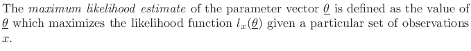
For the sinusoidal parameter estimation problem, given a set of
observed data samples ![]() , for
, for
![]() , the likelihood
function is
, the likelihood
function is
 |
(6.50) |
and the log likelihood function is
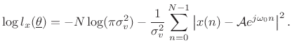 |
(6.51) |
We see that the maximum likelihood estimate for the parameters of a sinusoid in Gaussian white noise is the same as the least squares estimate. That is, given
 |
(6.52) |
as we saw before in (5.33).
Multiple Sinusoids in Additive Gaussian White Noise
The preceding analysis can be extended to the case of multiple sinusoids in white noise [120]. When the sinusoids are well resolved, i.e., when window-transform side lobes are negligible at the spacings present in the signal, the optimal estimator reduces to finding multiple interpolated peaks in the spectrum.
One exact special case is when the sinusoid frequencies ![]() coincide with the ``DFT frequencies''
coincide with the ``DFT frequencies''
![]() , for
, for
![]() . In this special case, each sinusoidal peak sits
atop a zero crossing in the window transform associated with every
other peak.
. In this special case, each sinusoidal peak sits
atop a zero crossing in the window transform associated with every
other peak.
To enhance the ``isolation'' among multiple sinusoidal peaks, it is natural to use a window function which minimizes side lobes. However, this is not optimal for short data records since valuable data are ``down-weighted'' in the analysis. Fundamentally, there is a trade-off between peak estimation error due to overlapping side lobes and that due to widening the main lobe. In a practical sinusoidal modeling system, not all sinusoidal peaks are recovered from the data--only the ``loudest'' peaks are measured. Therefore, in such systems, it is reasonable to assure (by choice of window) that the side-lobe level is well below the ``cut-off level'' in dB for the sinusoidal peaks. This prevents side lobes from being comparable in magnitude to sinusoidal peaks, while keeping the main lobes narrow as possible.
When multiple sinusoids are close together such that the associated main lobes overlap, the maximum likelihood estimator calls for a nonlinear optimization. Conceptually, one must search over the possible superpositions of the window transform at various relative amplitudes, phases, and spacings, in order to best ``explain'' the observed data.
Since the number of sinusoids present is usually not known, the number can be estimated by means of hypothesis testing in a Bayesian framework [21]. The ``null hypothesis'' can be ``no sinusoids,'' meaning ``just white noise.''
Non-White Noise
The noise process ![]() in (5.44) does not have to be white
[120]. In the non-white case, the spectral shape of the noise
needs to be estimated and ``divided out'' of the spectrum. That is, a
``pre-whitening filter'' needs to be constructed and applied to the
data, so that the noise is made white. Then the previous case can be
applied.
in (5.44) does not have to be white
[120]. In the non-white case, the spectral shape of the noise
needs to be estimated and ``divided out'' of the spectrum. That is, a
``pre-whitening filter'' needs to be constructed and applied to the
data, so that the noise is made white. Then the previous case can be
applied.
Generality of Maximum Likelihood Least Squares
Note that the maximum likelihood estimate coincides with the least squares estimate whenever the signal model is of the form
| (6.53) |
where
Next Section:
Spectrum Analysis of Noise
Previous Section:
FIR Digital Filter Design


