Rigid-Body Dynamics

Free Books Physical Audio Signal Processing

Below are selected topics from rigid-body dynamics, a subtopic of classical mechanics involving the use of Newton's laws of motion to solve for the motion of rigid bodies moving in 1D, 2D, or 3D space.^B.11 We may think of a rigid body as a distributed mass, that is, a mass that has length, area, and/or volume rather than occupying only a single point in space. Rigid body models have application in stiff strings (modeling them as disks of mass interconnect by ideal springs), rigid bridges, resonator braces, and so on.

We have already used Newton's to formulate mathematical dynamic models for the ideal point-mass (§B.1.1), spring (§B.1.3), and a simple mass-spring system (§B.1.4). Since many physical systems can be modeled as assemblies of masses and (normally damped) springs, we are pretty far along already. However, when the springs interconnecting our point-masses are very stiff, we may approximate them as rigid to simplify our simulations. Thus, rigid bodies can be considered mass-spring systems in which the springs are so stiff that they can be treated as rigid massless rods (infinite spring-constants , in the notation of §B.1.3).

So, what is new about distributed masses, as opposed to the point-masses considered previously? As we will see, the main new ingredient is rotational dynamics. The total momentum of a rigid body (distributed mass) moving through space will be described as the sum of the linear momentum of its center of mass (§B.4.1 below) plus the angular momentum about its center of mass (§B.4.13 below).

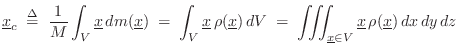
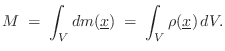
Center of Mass

The center of mass (or centroid) of a rigid body is found by averaging the spatial points of the body $\underline{x}_i\in{\bf R}^3$ weighted by the mass of those points:^B.12

$\displaystyle \underline{x}_c \isdefs \left. \sum_{i=1}^N m_i \underline{x}_i \right/ \sum_{i=1}^N m_i$

Thus, the center of mass is the mass-weighted average location of the object. For a continuous mass distribution totaling up to

, we can write

$\displaystyle \underline{x}_c \isdefs \frac{1}{M}\int_V \underline{x}\, dm(\un... ...p \iiint_{\underline{x}\in V} \underline{x}\, \rho(\underline{x})\, dx\,dy\,dz$

where the volume integral is taken over a volume

of 3D space that includes the rigid body, and $dm(\underline{x}) = m(\underline{x})dV = m(\underline{x})\, dx\,dy\,dz$ denotes the mass contained within the differential volume element

located at the point $\underline{x}\in{\bf R}^3$ , with $\rho(\underline{x})$ denoting the mass density at the point $\underline{x}$ . The total mass is

$\displaystyle M \eqsp \int_V dm(\underline{x}) \eqsp \int_V \rho(\underline{x})\, dV.$

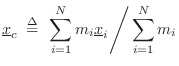
A nice property of the center of mass is that gravity acts on a far-away object as if all its mass were concentrated at its center of mass. For this reason, the center of mass is often called the center of gravity.

Linear Momentum of the Center of Mass

Consider a system of point-masses , each traveling with vector velocity $\underline{v}_i$ , and not necessarily rigidly attached to each other. Then the total momentum of the system is

$\displaystyle \underline{p}\eqsp \sum_{i=1}^N m_i \underline{v}_i \eqsp \sum_{... ...ine{x}_i \right) \eqsp M \frac{d}{dt} \underline{x}_c \isdef M \underline{v}_c$

where $M=\sum m_i$ denotes the total mass, and $\underline{v}_c$ is the velocity of the center of mass.

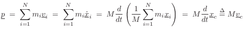
Thus, the momentum $\underline{p}$ of any collection of masses (including rigid bodies) equals the total mass times the velocity of the center-of-mass.

Whoops, No Angular Momentum!

The previous result might be surprising since we said at the outset that we were going to decompose the total momentum into a sum of linear plus angular momentum. Instead, we found that the total momentum is simply that of the center of mass, which means any angular momentum that might have been present just went away. (The center of mass is just a point that cannot rotate in a measurable way.) Angular momentum does not contribute to linear momentum, so it provides three new ``degrees of freedom'' (three new energy storage dimensions, in 3D space) that are ``missed'' when considering only linear momentum.

To obtain the desired decomposition of momentum into linear plus angular momentum, we will choose a fixed reference point in space (usually the center of mass) and then, with respect to that reference point, decompose an arbitrary mass-particle travel direction into the sum of two mutually orthogonal vector components: one will be the vector component pointing radially with respect to the fixed point (for the ``linear momentum'' component), and the other will be the vector component pointing tangentially with respect to the fixed point (for the ``angular momentum''), as shown in Fig.B.3. When the reference point is the center of mass, the resultant radial force component gives us the force on the center of mass, which creates linear momentum, while the net tangential component (times distance from the center-of-mass) give us a resultant torque about the reference point, which creates angular momentum. As we saw above, because the tangential force component does not contribute to linear momentum, we can simply sum the external force vectors and get the same result as summing their radial components. These topics will be discussed further below, after some elementary preliminaries.

**Figure:** Rigid body having center of mass at $\underline{0}$ , experiencing an external force $\underline{f}$ that can be expressed as the sum of radial and tangential components $\underline{f}=\underline{f}_r+\underline{f}_t$ . The radial component $\underline{f}_r$ accelerates the center-of-mass, while the tangential component $\underline{f}_t$ causes rotation about the center of mass.
$\includegraphics[width=1.5in]{eps/rigidbody}$

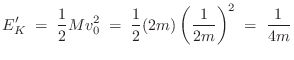
Translational Kinetic Energy

The translational kinetic energy of a collection of masses is given by

$\displaystyle E_K \eqsp \frac{1}{2} M v_c^2$

where $M=\sum_i m_i$ is the total mass, and

denotes the speed of the center-of-mass. We have $v_c\isdeftext \left\Vert\,\underline{v}_c\,\right\Vert$ , where $\underline{v}_c$ is the velocity of the center of mass.

More generally, the total energy of a collection of masses (including distributed and/or rigidly interconnected point-masses) can be expressed as the sum of the translational and rotational kinetic energies [270, p. 98].

Rotational Kinetic Energy

**Figure B.4:** Point-mass rotating in a circle of radius with tangential speed $v=R\omega$ , where $\omega=\dot{\theta}$ denotes the angular velocity in rad/s.
$\includegraphics[width=1.2in]{eps/masscircle}$

The rotational kinetic energy of a rigid assembly of masses (or mass distribution) is the sum of the rotational kinetic energies of the component masses. Therefore, consider a point-mass rotating^B.13 in a circular orbit of radius and angular velocity $\omega$ (radians per second), as shown in Fig.B.4. To make it a closed system, we can imagine an effectively infinite mass at the origin $\underline{0}$ . Then the speed of the mass along the circle is $v=R\omega$ , and its kinetic energy is $(1/2)mv^2=(1/2)mR^2\omega^2$ . Since this is what we want for the rotational kinetic energy of the system, it is convenient to define it in terms of angular velocity $\omega$ in radians per second. Thus, we write

$\displaystyle E_R \eqsp \frac{1}{2} I \omega^2, \protect$

(B.7)

where

$\displaystyle I \eqsp mR^2 \protect$

(B.8)

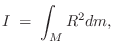
is called the mass moment of inertia.

Mass Moment of Inertia

The mass moment of inertia (or simply moment of inertia), plays the role of mass in rotational dynamics, as we saw in Eq. $\,$ (B.7) above.

The mass moment of inertia of a rigid body, relative to a given axis of rotation, is given by a weighted sum over its mass, with each mass-point weighted by the square of its distance from the rotation axis. Compare this with the center of mass (§B.4.1) in which each mass-point is weighted by its vector location in space (and divided by the total mass).

Equation (B.8) above gives the moment of inertia for a single point-mass rotating a distance from the axis to be . Therefore, for a rigid collection of point-masses , $i=1,\ldots,N$ ,^B.14 the moment of inertia about a given axis of rotation is obtained by adding the component moments of inertia:

$\displaystyle I = m_1 R_1^2 + m_2 R_2^2 + \cdots + m_N R_N^2, \protect$

(B.9)

where

is the distance from the axis of rotation to the

th mass.

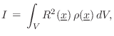
For a continuous mass distribution, the moment of inertia is given by integrating the contribution of each differential mass element:

$\displaystyle I \eqsp \int_M R^2 dm,$

(B.10)

where

is the distance from the axis of rotation to the mass element

. In terms of the density $\rho(\underline{x})$ of a continuous mass distribution, we can write

$\displaystyle I \,\mathrel{\mathop=}\,\int_V R^2(\underline{x})\,\rho(\underline{x})\,dV,$

where $\rho(\underline{x})$ denotes the mass density (kg/m $\null^3$ ) at the point $\underline{x}$ , and $dV=dx\,dy\,dz$ denotes a differential volume element located at $\underline{x}\in{\bf R}^3$ .

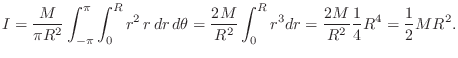
Circular Disk Rotating in Its Own Plane

For example, the moment of inertia for a uniform circular disk of total mass and radius , rotating in its own plane about a rotation axis piercing its center, is given by

$\displaystyle I = \frac{M}{\pi R^2}\int_{-\pi}^\pi \int_0^R r^2\, r\,dr\,d\thet... ...c{2M}{R^2}\int_0^R r^3 dr = \frac{2M}{R^2}\frac{1}{4} R^4 = \frac{1}{2} M R^2.$

Circular Disk Rotating About Its Diameter

The moment of inertia for the same circular disk rotating about an axis in the plane of the disk, passing through its center, is given by

$\displaystyle I = \frac{M}{\pi R^2}\cdot 4\int_0^{\pi/2} \int_0^R [r\cos(\theta)]^2\, r\,dr\,d\theta = \frac{1}{4}MR^2$

Thus, the uniform disk's moment of inertia in its own plane is twice that about its diameter.

Perpendicular Axis Theorem

In general, for any 2D distribution of mass, the moment of inertia about an axis orthogonal to the plane of the mass equals the sum of the moments of inertia about any two mutually orthogonal axes in the plane of the mass intersecting the first axis. To see this, consider an arbitrary mass element having rectilinear coordinates in the plane of the mass. (All three coordinate axes intersect at a point in the mass-distribution plane.) Then its moment of inertia about the axis orthogonal to the mass plane is $dm\,(x_1^2+x_2^2)$ while its moment of inertia about coordinate axes within the mass-plane are respectively $dm\,x_1^2$ and $dm\,x_2^2$ . This, the perpendicular axis theorem is an immediate consequence of the Pythagorean theorem for right triangles.

Parallel Axis Theorem

Let denote the moment of inertia for a rotation axis passing through the center of mass, and let denote the moment of inertia for a rotation axis parallel to the first but a distance away from it. Then the parallel axis theorem says that

$\displaystyle I_d = I_0 + Md^2$

where

denotes the total mass. Thus, the added inertia due to displacement by

meters away from the centroidal axis is equal to that of a point mass

rotating a distance

from the center of rotation.

Stretch Rule

Note that the moment of inertia does not change when masses are moved along a vector parallel to the axis of rotation (see, e.g., Eq. $\,$ (B.9)). Thus, any rigid body may be ``stretched'' or ``squeezed'' parallel to the rotation axis without changing its moment of inertia. This is known as the stretch rule, and it can be used to simplify geometry when finding the moment of inertia.

For example, we saw in §B.4.4 that the moment of inertia of a point-mass a distance from the axis of rotation is given by . By the stretch rule, the same applies to an ideal rod of mass parallel to and distance from the axis of rotation.

Note that mass can be also be ``stretched'' along the circle of rotation without changing the moment of inertia for the mass about that axis. Thus, the point mass can be stretched out to form a mass ring at radius about the axis of rotation without changing its moment of inertia about that axis. Similarly, the ideal rod of the previous paragraph can be stretched tangentially to form a cylinder of radius and mass , with its axis of symmetry coincident with the axis of rotation. In all of these examples, the moment of inertia is about the axis of rotation.

Area Moment of Inertia

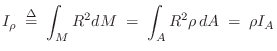
The area moment of inertia is the second moment of an area around a given axis:

$\displaystyle I_A = \int_A R^2(\underline{x}) dA$

where

denotes a differential element of the area (summing to

), and $R(\underline{x})$ denotes its distance from the axis of rotation.

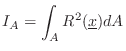
Comparing with the definition of mass moment of inertia in §B.4.4 above, we see that mass is replaced by area in the area moment of inertia.

In a planar mass distribution with total mass uniformly distributed over an area (i.e., a constant mass density of $\rho=M/A$ ), the mass moment of inertia $I_\rho$ is given by the area moment of inertia times mass-density $\rho$ :

$\displaystyle I_\rho \isdefs \int_M R^2 dM \eqsp \int_A R^2 \rho\, dA \eqsp \rho I_A$

Radius of Gyration

For a planar distribution of mass rotating about some axis in the plane of the mass, the radius of gyration is the distance from the axis that all mass can be concentrated to obtain the same mass moment of inertia. Thus, the radius of gyration is the ``equivalent distance'' of the mass from the axis of rotation. In this context, gyration can be defined as rotation of a planar region about some axis lying in the plane.

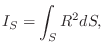
For a bar cross-section with area , the radius of gyration is given by

$\displaystyle R_g = \sqrt{\frac{I_S}{S}} \protect$

(B.11)

where

is the area moment of inertia (§B.4.8) of the cross-section about a given axis of rotation lying in the plane of the cross-section (usually passing through its centroid):

$\displaystyle I_S = \int_S R^2 dS,$

where

denotes the distance of the differential area element

from the axis of gyration.

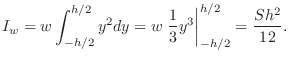
Rectangular Cross-Section

For a rectangular cross-section of height and width , area , the area moment of inertia about the horizontal midline is given by

$\displaystyle I_w = w\int_{-h/2}^{h/2} y^2 dy = w\left.\frac{1}{3}y^3\right\vert _{-h/2}^{h/2} = \frac{Sh^2}{12}.$

The radius of gyration about this axis is then

$\displaystyle R_g = \sqrt{\frac{I_w}{S}} = \sqrt{\frac{h^2}{12}} = \frac{h}{2\sqrt{3}}.$

Similarly, the radius of gyration about a vertical axis passing through the center of the cross-section is $R_g=w/(2\sqrt{3})$ .

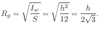
The radius of gyration can be thought of as the ``effective radius'' of the mass distribution with respect to its inertial response to rotation (``gyration'') about the chosen axis.

Most cross-sectional shapes (e.g., rectangular), have at least two radii of gyration. A circular cross-section has only one, and its radius of gyration is equal to half its radius, as shown in the next section.

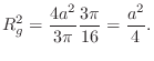
Circular Cross-Section

For a circular cross-section of radius , Eq. $\,$ (B.11) tells us that the squared radius of gyration about any line passing through the center of the cross-section is given by

$\begin{eqnarray*} R_g^2 &=& \frac{1}{\pi a^2} \int_{-a}^a dx \int_{-\sqrt{a^2-x^... ...frac{4a^2}{3\pi} \int_{0}^{\frac{\pi}{2}} \cos^4(\theta)d\theta. \end{eqnarray*}$

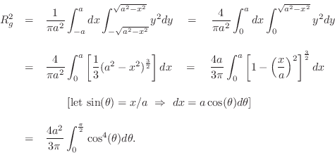
Using the elementrary trig identity $\cos(2\theta)=2\cos^2(\theta)-1$ , we readily derive

$\displaystyle \cos^4(\theta) = \frac{1}{8}\cos(4\theta) + \frac{1}{2}\cos(2\theta) + \frac{3}{8}.$

The first two terms of this expression contribute zero to the integral from 0 to $\pi /2$ , while the last term contributes $3\pi/16$ , yielding

$\displaystyle R_g^2 = \frac{4a^2}{3\pi} \frac{3\pi}{16} = \frac{a^2}{4}.$

Thus, the radius of gyration about any midline of a circular cross-section of radius

$\displaystyle R_g = \frac{a}{2}.$

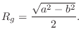
For a circular tube in which the mass of the cross-section lies within a circular annulus having inner radius and outer radius , the radius of gyration is given by

$\displaystyle R_g = \frac{\sqrt{a^2-b^2}}{2}. \protect$

(B.12)

Two Masses Connected by a Rod

**Figure B.5:** Two ideal point-masses connected by an ideal, rigid, massless rod of length .
$\includegraphics[width=1.5in]{eps/massrodmass}$

As an introduction to the decomposition of rigid-body motion into translational and rotational components, consider the simple system shown in Fig.B.5. The excitation force density^B.15 can be applied anywhere between and along the connecting rod. We will deliver a vertical impulse of momentum to the mass on the right, and show, among other observations, that the total kinetic energy is split equally into (1) the rotational kinetic energy about the center of mass, and (2) the translational kinetic energy of the total mass, treated as being located at the center of mass. This is accomplished by defining a new frame of reference (i.e., a moving coordinate system) that has its origin at the center of mass.

First, note that the driving-point impedance (§7.1) ``seen'' by the driving force varies as a function of . At , The excitation sees a ``point mass'' , and no rotation is excited by the force (by symmetry). At $x=\pm R$ , on the other hand, the excitation $f(t,\pm R)dx$ only sees mass at time 0, because the vertical motion of either point-mass initially only rotates the other point-mass via the massless connecting rod. Thus, an observation we can make right away is that the driving point impedance seen by depends on the striking point and, away from , it depends on time as well.

To avoid dealing with a time-varying driving-point impedance, we will use an impulsive force input at time . Since momentum is the time-integral of force ( $f=ma=m\dot{v}\,\,\Rightarrow\,\,mv=\int f\,dt$ ), our excitation will be a unit momentum transferred to the two-mass system at time 0.

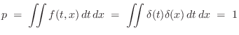
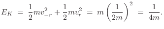
Striking the Rod in the Middle

First, consider $f(t,x)=\delta(t)\delta(x)$ . That is, we apply an upward unit-force impulse at time 0 in the middle of the rod. The total momentum delivered in the neighborhood of and is obtained by integrating the applied force density with respect to time and position:

$\displaystyle p \eqsp \iint f(t,x)\,dt\,dx \eqsp \iint \delta(t)\delta(x)\,dt\,dx \eqsp 1$

This unit momentum is transferred to the two masses

. By symmetry, we have $v_{-r} = v_r = v_0$ . We can also refer to

as the velocity of the center of mass, again obvious by symmetry. Continuing to refer to Fig.B.5, we have

$\displaystyle p \eqsp 1 \eqsp mv_{-r} + mv_r \eqsp (2m)v_0 \,\,\Rightarrow\,\,v_0 \eqsp \frac{1}{2m}.$

Thus, after time zero, each mass is traveling upward at speed

, and there is no rotation about the center of mass at

The kinetic energy of the system after time zero is

$\displaystyle E_K \eqsp \frac{1}{2} mv_{-r}^2 + \frac{1}{2}mv_r^2 \eqsp m\left(\frac{1}{2m}\right)^2 \eqsp \frac{1}{4m}.$

Note that we can also compute

in terms of the total mass

and the velocity of the center of mass

$\displaystyle E_K \eqsp \frac{1}{2} Mv_0^2 \eqsp \frac{1}{2} (2m)\left(\frac{1}{2m}\right)^2 \eqsp \frac{1}{4m}$

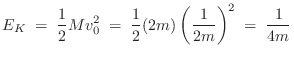
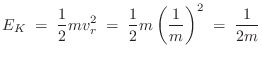
Striking One of the Masses

Now let $f(t,x) = \delta(t)\delta(x-r)$ . That is, we apply an impulse of vertical momentum to the mass on the right at time 0.

In this case, the unit of vertical momentum is transferred entirely to the mass on the right, so that

$\displaystyle p \eqsp 1 \eqsp m v_r \,\,\Rightarrow\,\,v_r \eqsp \frac{1}{m},$

which is twice as fast as before. Just after time zero, we have

, $v_{-r}=0$ , and, because the massless rod remains rigid,

Note that the velocity of the center-of-mass is the same as it was when we hit the midpoint of the rod. This is an important general equivalence: The sum of all external force vectors acting on a rigid body can be applied as a single resultant force vector to the total mass concentrated at the center of mass to find the linear (translational) motion produced. (Recall from §B.4.1 that such a sum is the same as the sum of all radially acting external force components, since the tangential components contribute only to rotation and not to translation.)

All of the kinetic energy is in the mass on the right just after time zero:

$\displaystyle E_K \eqsp \frac{1}{2}mv_r^2 \eqsp \frac{1}{2}m\left(\frac{1}{m}\right)^2 \eqsp \frac{1}{2m} \protect$

(B.13)

However, after time zero, things get more complicated, because the mass on the left gets dragged into a rotation about the center of mass.

To simplify ongoing analysis, we can define a body-fixed frame of reference^B.16 having its origin at the center of mass. Let denote a velocity in this frame. Since the velocity of the center of mass is , we can convert any velocity in the body-fixed frame to a velocity in the original frame by adding to it, viz.,

$\displaystyle v \eqsp v' + v_0 \eqsp v' + \frac{1}{2m}.$

The mass velocities in the body-fixed frame are now

$\displaystyle v'_{-r} \eqsp -\frac{1}{2m},\qquad\qquad v'_r \eqsp \frac{1}{2m},$

and of course

In the body-fixed frame, all kinetic energy is rotational about the origin. Recall (Eq. $\,$ (B.9)) that the moment of inertia for this system, with respect to the center of mass at , is

$\displaystyle I \eqsp m(-r)^2 + m r^2 \eqsp 2mr^2.$

Thus, the rotational kinetic energy (§B.4.3) is found to be

$\displaystyle E'_R \eqsp \frac{1}{2}I\omega^2 \eqsp \frac{1}{2}(2mr^2)\left(\frac{v'_r}{r}\right)^2 \eqsp mr^2\left(\frac{1}{2mr}\right)^2 \eqsp \frac{1}{4m}.$

This is half of the kinetic energy we computed in the original ``space-fixed'' frame (Eq. $\,$ (B.13) above). The other half is in the translational kinetic energy not seen in the body-fixed frame. As we saw in §B.4.2 above, we can easily calculate the translational kinetic energy as that of the total mass

traveling at the center-of-mass velocity

$\displaystyle E'_K \eqsp \frac{1}{2}Mv_0^2 \eqsp \frac{1}{2}(2m)\left(\frac{1}{2m}\right)^2 \eqsp \frac{1}{4m}$

Adding this translational kinetic energy to the rotational kinetic energy in the body-fixed frame yields the total kinetic energy, as it must.

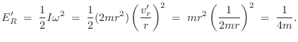
In summary, we defined a moving body-fixed frame having its origin at the center-of-mass, and the total kinetic energy was computed to be

$\displaystyle E_K \eqsp E'_K + E'_R \eqsp \frac{1}{4m} + \frac{1}{4m} \eqsp \frac{1}{2m}$

in agreement with the more complicated (after time zero) space-fixed analysis in Eq. $\,$ (B.13).

It is important to note that, after time zero, both the linear momentum of the center-of-mass ( $p_0=Mv_0=(2m)(v_r/2) = mv_r=m\cdot(1/(2m))=1/2$ ), and the angular momentum in the body-fixed frame ( $L'=I\omega= (2mr^2)(v'_r/r)=(2mr^2)(1/(2mr))=r/2$ ) remain constant over time.^B.17 In the original space-fixed frame, on the other hand, there is a complex transfer of momentum back and forth between the masses after time zero.

Similarly, the translational kinetic energy of the total mass, treated as being concentrated at its center-of-mass, and the rotational kinetic energy in the body-fixed frame, are both constant after time zero, while in the space-fixed frame, kinetic energy transfers back and forth between the two masses. At all times, however, the total kinetic energy is the same in both formulations.

Angular Velocity Vector

When working with rotations, it is convenient to define the angular-velocity vector as a vector $\underline{\omega}\in{\bf R}^3$ pointing along the axis of rotation. There are two directions we could choose from, so we pick the one corresponding to the right-hand rule, i.e., when the fingers of the right hand curl in the direction of the rotation, the thumb points in the direction of the angular velocity vector.^B.18 The length $\vert\vert\,\underline{\omega}\,\vert\vert$ should obviously equal the angular velocity $\omega$ . It is convenient also to work with a unit-length variant $\underline{\tilde{\omega}}\isdeftext \underline{\omega}/ \vert\vert\,\underline{\omega}\,\vert\vert$ .

As introduced in Eq. $\,$ (B.8) above, the mass moment of inertia is given by where is the distance from the (instantaneous) axis of rotation to the mass located at $\underline{x}\in{\bf R}^3$ . In terms of the angular-velocity vector $\underline{\omega}$ , we can write this as (see Fig.B.6)

$\displaystyle I$	$\displaystyle =$	$\displaystyle mR^2 \eqsp m\cdot \left\Vert\,\underline{x}-{\cal P}_{\underline{\omega}}(\underline{x})\,\right\Vert^2$
	$\displaystyle =$	$\displaystyle m\cdot \left\Vert\,\underline{x}-(\underline{\tilde{\omega}}^T\underline{x})\underline{\tilde{\omega}}\,\right\Vert^2 \protect$	(B.14)

where

$\displaystyle {\cal P}_{\underline{\omega}}(\underline{x}) \isdefs \frac{\under... ...ga}\eqsp (\underline{\tilde{\omega}}^T\underline{x})\underline{\tilde{\omega}}$

denotes the orthogonal projection of $\underline{x}$ onto $\underline{\omega}$ (or $\underline{\tilde{\omega}}$ ) [451]. Thus, we can project the mass position $\underline{x}$ onto the angular-velocity vector $\underline{\omega}$ and subtract to get the component of $\underline{x}$ that is orthogonal to $\underline{\omega}$ , and the length of that difference vector is the distance to the rotation axis

, as shown in Fig.B.6.

**Figure:** Mass position vector $\underline{x}$ and its orthogonal projection ${\cal P}_{\protect\underline{\omega}}(\underline{x})$ onto the angular velocity vector $\underline{\omega}$ for purposes of finding the distance of the mass from the axis of rotation $\underline{\tilde{\omega}}$ .
$\includegraphics[width=1.5in]{eps/pxov}$

Using the vector cross product (defined in the next section), we will show (in §B.4.17) that can be written more succinctly as

$\displaystyle R \eqsp \left\Vert\,\underline{x}-{\cal P}_{\underline{\omega}}(\... ...\eqsp \left\Vert\,\underline{\tilde{\omega}}\times \underline{x}\,\right\Vert.$

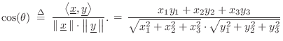
Vector Cross Product

The vector cross product (or simply vector product, as opposed to the scalar product (which is also called the dot product, or inner product)) is commonly used in vector calculus--a basic mathematical toolset used in mechanics [270,258], acoustics [349], electromagnetism [356], quantum mechanics, and more. It can be defined symbolically in the form of a matrix determinant:^B.19

$\displaystyle \underline{x}\times \underline{y}$	$\displaystyle =$	$\displaystyle \left\vert \begin{array}{ccc} \underline{e}_1 & \underline{e}_2 &... ...ine{e}_3\\ [2pt] x_1 & x_2 & x_3\\ [2pt] y_1 & y_2 & y_3 \end{array}\right\vert$
	$\displaystyle =$	$\displaystyle (x_2 y_3 - y_2 x_3)\underline{e}_1 + (x_3y_1 - y_3x_1) \underline{e}_2 + (x_1y_2- y_1x_2) \underline{e}_3$
	$\displaystyle =$	$\displaystyle \left[\begin{array}{ccc} 0 & -x_3 & x_2\\ [2pt] x_3 & 0 & -x_1\\ ... ...}\right] \left[\begin{array}{c} x_1 \\ [2pt] x_2 \\ [2pt] x_3\end{array}\right]$
		$\displaystyle \protect$	(B.15)

where $\underline{e}_i$ denote the unit vectors in ${\bf R}^3$ . The cross-product is a vector in 3D that is orthogonal to the plane spanned by $\underline{x}$ and $\underline{y}$ , and is oriented positively according to the right-hand rule.^B.20

The second and third lines of Eq. $\,$ (B.15) make it clear that $y\times x = -\; x\times y$ . This is one example of a host of identities that one learns in vector calculus and its applications.

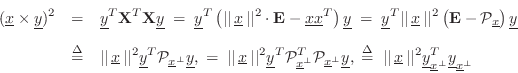
Cross-Product Magnitude

It is a straightforward exercise to show that the cross-product magnitude is equal to the product of the vector lengths times the sine of the angle between them:^B.21

$\displaystyle \left\Vert\,\underline{x}\times \underline{y}\,\right\Vert \eqsp ... ...dot\left\Vert\,\underline{y}\,\right\Vert \cdot \vert\sin(\theta)\vert \protect$

(B.16)

where

$\displaystyle \sin(\theta)\eqsp \sqrt{1-\cos^2(\theta)}$

with

$\displaystyle \cos(\theta) \isdefs \frac{\left<\underline{x},\underline{y}\rig... ...c{x_1y_1+x_2y_2+x_3y_3}{\sqrt{x_1^2+x_2^2+x_3^2}\cdot\sqrt{y_1^2+y_2^2+y_3^2}}$

(Recall that the vector cosine of the angle between two vectors is given by their inner product divided by the product of their norms [451].)

To derive Eq. $\,$ (B.16), let's begin with the cross-product in matrix form as $\underline{x}\times\underline{y}= \mathbf{X}\underline{y}$ using the first matrix form in the third line of the cross-product definition in Eq. $\,$ (B.15) above. Then

$\begin{eqnarray*} (\underline{x}\times\underline{y})^2 &=& \underline{y}^T\mat... ...rline{x}^{\tiny\perp}}\underline{y}_{\underline{x}^{\tiny\perp}} \end{eqnarray*}$

where $\mathbf{E}=[\underline{e}_1,\underline{e}_2,\underline{e}_3]$ denotes the identity matrix in ${\bf R}^3$ , ${\cal P}_{\underline{x}}$ denotes the orthogonal-projection matrix onto $\underline{x}$ [451], ${\cal P}_{\underline{x}}$ denotes the projection matrix onto the orthogonal complement of $\underline{x}$ , $\underline{y}_{\underline{x}^{\tiny\perp}}$ denotes the component of $\underline{y}$ orthogonal to $\underline{x}$ , and we used the fact that orthogonal projection matrices ${\cal P}$ are idempotent (i.e., ${\cal P}^2 ={\cal P}$ ) and symmetric (when real, as we have here) when we replaced ${\cal P}_{\underline{x}^{\tiny\perp}}$ by ${\cal P}^T_{\underline{x}^{\tiny\perp}}{\cal P}_{\underline{x}^{\tiny\perp}}$ above. Finally, note that the length of $\underline{y}_{\underline{x}^{\tiny\perp}}$ is $\vert\vert\,\underline{y}\,\vert\vert \cdot\vert\sin(\theta)\vert$ , where $\theta$ is the angle between the 1D subspaces spanned by $\underline{x}$ and $\underline{y}$ in the plane including both vectors. Thus,

$\displaystyle (\underline{x}\times\underline{y})^2 \eqsp \vert\vert\,\underline... ...line{x}\,\vert\vert ^2 \vert\vert\,\underline{y}\,\vert\vert ^2\sin^2(\theta),$

which establishes the desired result:

$\displaystyle \left\Vert\,\underline{x}\times\underline{y}\,\right\Vert = \vert... ...t\vert \cdot \vert\vert\,\underline{y}\,\vert\vert \cdot\vert\sin(\theta)\vert$

Moreover, this proof gives an appealing geometric interpretation of the vector cross-product $\underline{x}\times\underline{y}$ as having magnitude given by the product of $\vert\vert\,\underline{x}\,\vert\vert$ times the norm of the difference between $\underline{x}$ and the orthogonal projection of $\underline{x}$ onto $\underline{y}$ ( $\vert\vert\,\underline{x}\times\underline{y}\,\vert\vert = \vert\vert\,\underl... ... \vert\vert\,\underline{x}-{\cal P}_{\underline{y}}(\underline{x})\,\vert\vert$ ) or vice versa ( $\vert\vert\,\underline{x}\times\underline{y}\,\vert\vert = \vert\vert\,\underl... ... \vert\vert\,\underline{y}-{\cal P}_{\underline{x}}(\underline{y})\,\vert\vert$ ). In this geometric picture it is clear that the cross-product magnitude is maximized when the vectors are orthogonal, and it is zero when the vectors are collinear. It is ``length times orthogonal length.''

The direction of the cross-product vector is then taken to be orthogonal to both $\underline{x}$ and $\underline{y}$ according to the right-hand rule. This orthogonality can be checked by verifying that $\mathbf{X}\underline{x}=\mathbf{Y}\underline{y}=\underline{0}$ . The right-hand-rule parity can be checked by rotating the space so that $\underline{x}'=[ \vert\vert\,\underline{x}\,\vert\vert ,0,0]^T$ and $\underline{y}'=[ \vert\vert\,\underline{y}\,\vert\vert \cos(\theta), \vert\vert\,\underline{y}\,\vert\vert \sin(\theta),0]^T$ in which case $\underline{x}'\times\underline{y}' = \vert\vert\,\underline{x}\,\vert\vert [0,... ...}\,\vert\vert \vert\vert\,\underline{y}\,\vert\vert \sin(\theta)\underline{e}_3$ . Thus, the cross product points ``up'' relative to the $(\underline{x},\underline{y})$ plane for $\theta \in(0,\pi)$ and ``down'' for $\theta\in(0,-\pi)$ .

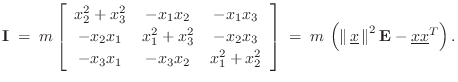
Mass Moment of Inertia as a Cross Product

In Eq. $\,$ (B.14) above, the mass moment of inertia was expressed in terms of orthogonal projection as $I = mR^2 = m\cdot \vert\vert\,\underline{x}-{\cal P}_{\underline{\omega}}(\und... ...erline{\tilde{\omega}}^T\underline{x})\underline{\tilde{\omega}}\,\vert\vert ^2$ , where $\underline{\tilde{\omega}}\isdeftext \underline{\omega}/ \vert\vert\,\underline{\omega}\,\vert\vert$ . In terms of the vector cross product, we can now express it as

$\displaystyle I \eqsp m\cdot(\underline{\tilde{\omega}}\times \underline{x})^2 ... ...cdot\sin(\theta_{\underline{\tilde{\omega}}\underline{x}})\right]^2 \eqsp mR^2$

where $R= \vert\vert\,\underline{x}\,\vert\vert \sin(\theta_{\underline{\tilde{\omega}}\underline{x}})$ is the distance from the rotation axis out to the point $\underline{x}$ (which equals the length of the vector $\underline{x}-{\cal P}_{\underline{\omega}}(\underline{x})$ ).

Tangential Velocity as a Cross Product

Referring again to Fig.B.4, we can write the tangential velocity vector $\underline{v}$ as a vector cross product of the angular-velocity vector $\underline{\omega}$ (§B.4.11) and the position vector $\underline{x}$ :

$\displaystyle \underline{v}\eqsp \underline{\omega}\times \underline{x} \protect$

(B.17)

To see this, let's first check its direction and then its magnitude. By the right-hand rule, $\underline{\omega}$ points up out of the page in Fig.B.4. Crossing that with $\underline{x}$ , again by the right-hand rule, produces a tangential velocity vector $\underline{v}$ pointing as shown in the figure. So, the direction is correct. Now, the magnitude: Since $\underline{\omega}$ and $\underline{x}$ are mutually orthogonal, the angle between them is $\pi /2$ , so that, by Eq. $\,$ (B.16),

$\displaystyle \left\Vert\,\underline{\omega}\times \underline{x}\,\right\Vert \... ...,\right\Vert\cdot\left\Vert\,\underline{x}\,\right\Vert \eqsp \omega R \eqsp v$

as desired.

Angular Momentum

The angular momentum of a mass rotating in a circle of radius with angular velocity $\omega$ (rad/s), is defined by

$\displaystyle L \eqsp I\omega$

where

denotes the mass moment of inertia of the rigid body (§B.4.4).

Relation of Angular to Linear Momentum

Recall (§B.3) that the momentum of a mass traveling with velocity in a straight line is given by

$\displaystyle p = m v,$

while the angular momentum of a point-mass

rotating along a circle of radius

at $\omega$ rad/s is given by

$\displaystyle L \eqsp I\omega,$

where

. The tangential speed of the mass along the circle of radius

is given by

$\displaystyle v \eqsp R\omega.$

Expressing the angular momentum

in terms of

gives

$\displaystyle L \isdefs I\omega \eqsp I\frac{v}{R} \isdefs mR^2\frac{v}{R} \eqsp Rmv \eqsp Rp. \protect$

(B.18)

Thus, the angular momentum

times the linear momentum

Linear momentum can be viewed as a renormalized special case of angular momentum in which the radius of rotation goes to infinity.

Angular Momentum Vector

Like linear momentum, angular momentum is fundamentally a vector in ${\bf R}^3$ . The definition of the previous section suffices when the direction does not change, in which case we can focus only on its magnitude $L=I\omega$ .

More generally, let $\underline{x}_m\in{\bf R}^3$ denote the 3-space coordinates of a point-mass , and let $\underline{v}_m=\dot{\underline{x}}_m$ denote its velocity in ${\bf R}^3$ . Then the instantaneous angular momentum vector of the mass relative to the origin (not necessarily rotating about a fixed axis) is given by

$\displaystyle \underline{L}\isdefs m\, \underline{x}_m \times \underline{v}_m \eqsp m\, \underline{x}_m \times (\underline{\omega}\times\underline{x}_m) \protect$

(B.19)

where $\times$ denotes the vector cross product, discussed in §B.4.12 above. The identity $\underline{v}_m=\underline{\omega}\times\underline{x}_m$ was discussed at Eq. $\,$ (B.17).

For the special case in which $\underline{v}_m$ is orthogonal to $\underline{x}_m$ , as in Fig.B.4, we have that $x_m\times\underline{v}_m$ points, by the right-hand rule, in the direction of the angular velocity vector $\underline{\omega}$ (up out of the page), which is satisfying. Furthermore, its magnitude is given by

$\displaystyle \left\Vert\,\underline{L}\,\right\Vert \eqsp m\left\Vert\,\underl... ...ft\Vert\,\underline{v}_m\,\right\Vert \eqsp mRv \eqsp mR^2\omega \eqsp I\omega$

which agrees with the scalar case.

In the more general case of an arbitrary mass velocity vector $\underline{v}_m$ , we know from §B.4.12 that the magnitude of $\underline{x}_m\times\underline{v}_m$ equals the product of the distance from the axis of rotation to the mass, i.e., $\vert\vert\,\underline{x}_m\,\vert\vert$ , times the length of the component of $\underline{v}_m$ that is orthogonal to $\underline{x}$ , i.e., $\vert\vert\,\underline{v}_m\,\vert\vert \sin(\theta)$ , as needed.

It can be shown that vector angular momentum, as defined, is conserved.^B.22 For example, in an orbit, such as that of the moon around the earth, or that of Halley's comet around the sun, the orbiting object speeds up as it comes closer to the object it is orbiting. (See Kepler's laws of planetary motion.) Similarly, a spinning ice-skater spins faster when pulling in arms to reduce the moment of inertia about the spin axis. The conservation of angular momentum can be shown to result from the principle of least action and the isotrophy of space [270, p. 18].

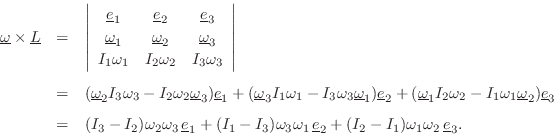
Angular Momentum Vector in Matrix Form

The two cross-products in Eq. $\,$ (B.19) can be written out with the help of the vector analysis identity^B.23

$\displaystyle \underline{x}\times (\underline{y}\times\underline{z}) \eqsp \und... ...underline{z}^T\underline{x})-\underline{z}\cdot(\underline{x}^T\underline{y}).$

This (or a direct calculation) yields, starting with Eq. $\,$ (B.19),

$\displaystyle \underline{L}$	$\displaystyle =$	$\displaystyle m\, \underline{x}_m \times (\underline{\omega}\times\underline{x}... ...line{x}^T\underline{x}) - \underline{x}\cdot(\underline{x}^T\underline{\omega})$
	$\displaystyle =$	$\displaystyle m\,\left(\left\Vert\,\underline{x}\,\right\Vert^2\mathbf{E}- \underline{x}\underline{x}^T\right)\underline{\omega}$
	$\displaystyle \isdef$	$\displaystyle \mathbf{I}\,\underline{\omega} \protect$	(B.20)

where

$\displaystyle \mathbf{I}\underline{\omega}\eqsp \left[\begin{array}{ccc} I_{1... ...begin{array}{c} \omega_1 \\ [2pt] \omega_2 \\ [2pt] \omega_3\end{array}\right]$

with $I_{ii}=m\left(\sum_{j=1}^3x_j^2 - x_i^2\right)$ , and $I_{ij}=-mx_ix_j$ , for $i\ne j$ . That is,

$\displaystyle \mathbf{I}\eqsp m\left[\begin{array}{ccc} x_2^2+x_3^2 & -x_1x_2 &... ...line{x}\,\right\Vert^2\mathbf{E}- \underline{x}\underline{x}^T\right). \protect$

(B.21)

The matrix $\mathbf{I}$ is the Cartesian representation of the mass moment of inertia tensor, which will be explored further in §B.4.15 below.

The vector angular momentum of a rigid body is obtained by summing the angular momentum of its constituent mass particles. Thus,

$\displaystyle \underline{L}\eqsp \sum_i m_i \left(\left\Vert\,\underline{x}_i\,... ...e{x}_i^T\right)\underline{\omega} \,\isdefs \, \mathbf{I}\,\underline{\omega}.$

Since $\underline{\omega}$ factors out of the sum, we see that the mass moment of inertia tensor for a rigid body is given by the sum of the mass moment of inertia tensors for each of its component mass particles.

In summary, the angular momentum vector $\underline{L}$ is given by the mass moment of inertia tensor $\mathbf{I}$ times the angular-velocity vector $\underline{\omega}$ representing the axis of rotation.

Note that the angular momentum vector $\underline{L}$ does not in general point in the same direction as the angular-velocity vector $\underline{\omega}$ . We saw above that it does in the special case of a point mass traveling orthogonal to its position vector. In general, $\underline{L}$ and $\underline{\omega}$ point in the same direction whenever $\underline{\omega}$ is an eigenvector of $\mathbf{I}$ , as will be discussed further below (§B.4.16). In this case, the rigid body is said to be dynamically balanced.^B.24

Mass Moment of Inertia Tensor

As derived in the previous section, the moment of inertia tensor, in 3D Cartesian coordinates, is a three-by-three matrix $\mathbf{I}$ that can be multiplied by any angular-velocity vector to produce the corresponding angular momentum vector for either a point mass or a rigid mass distribution. Note that the origin of the angular-velocity vector $\underline{\omega}$ is always fixed at $\underline{0}$ in the space (typically located at the center of mass). Therefore, the moment of inertia tensor $\mathbf{I}$ is defined relative to that origin.

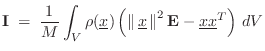
The moment of inertia tensor can similarly be used to compute the mass moment of inertia for any normalized angular velocity vector $\underline{\tilde{\omega}}=\underline{\omega}/ \vert\vert\,\underline{\omega}\,\vert\vert$ as

$\displaystyle I \eqsp \underline{\tilde{\omega}}^T\mathbf{I}\,\underline{\tilde{\omega}}. \protect$

(B.22)

Since rotational energy is defined as $(1/2)I\omega^2$ (see Eq. $\,$ (B.7)), multiplying Eq. $\,$ (B.22) by $\omega^2$ gives the following expression for the rotational kinetic energy in terms of the moment of inertia tensor:

$\displaystyle E_R \eqsp \frac{1}{2}\, \underline{\omega}^T\mathbf{I}\,\underline{\omega} \protect$

(B.23)

We can show Eq. $\,$ (B.22) starting from Eq. $\,$ (B.14). For a point-mass

located at $\underline{x}$ , we have

$\begin{eqnarray*} I &=& m \left\Vert\,\underline{x}-(\underline{\tilde{\omega}}^... ...nderline{\tilde{\omega}}^T\mathbf{I}\,\underline{\tilde{\omega}} \end{eqnarray*}$

where again $\mathbf{E}$ denotes the three-by-three identity matrix, and

$\displaystyle \mathbf{I}\eqsp m \left(\left\Vert\,\underline{x}\,\right\Vert^2\mathbf{E}-\underline{x}\underline{x}^T\right), \protect$

(B.24)

which agrees with Eq. $\,$ (B.20). Thus we have derived the moment of inertia

in terms of the moment of inertia tensor $\mathbf{I}$ and the normalized angular velocity $\underline{\tilde{\omega}}$ for a point-mass

at $\underline{x}$ .

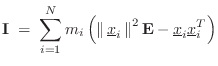
For a collection of masses located at $\underline{x}_i\in{\bf R}^3$ , we simply sum over their masses to add up the moments of inertia:

$\displaystyle \mathbf{I}\eqsp \sum_{i=1}^N m_i \left(\left\Vert\,\underline{x}_i\,\right\Vert^2\mathbf{E} -\underline{x}_i\underline{x}_i^T\right)$

Finally, for a continuous mass distribution, we integrate as usual:

$\displaystyle \mathbf{I}\eqsp \frac{1}{M}\int_V \rho(\underline{x}) \left(\left... ...underline{x}\,\right\Vert^2\mathbf{E} -\underline{x}\underline{x}^T\right)\,dV$

where $M=\int_V\rho(\underline{x})dV$ is the total mass.

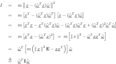
Simple Example

Consider a mass at $\underline{x}=[x,0,0]^T$ . Then the mass moment of inertia tensor is

$\displaystyle \mathbf{I}\eqsp m \left(\left\Vert\,\underline{x}\,\right\Vert^2\... ...ay}{ccc} 0 & 0 & 0\\ [2pt] 0 & 1 & 0\\ [2pt] 0 & 0 & 1 \end{array}\right].$

For the angular-velocity vector $\underline{\omega}=[\omega,0,0]^T$ , we obtain the moment of inertia

$\begin{displaymath} I \eqsp \underline{\tilde{\omega}}^T\mathbf{I}\,\underline{\... ...{array}{c} 1 \\ [2pt] 0 \\ [2pt] 0\end{array}\right]m \eqsp 0. \end{displaymath}$

This makes sense because the axis of rotation passes through the point mass, so the moment of inertia should be zero about that axis. On the other hand, if we look at $\underline{\omega}=[0,1,0]^T$ , we get

$\displaystyle I \eqsp \underline{\tilde{\omega}}^T\mathbf{I}\,\underline{\tilde... ...] \left[\begin{array}{c} 0 \\ [2pt] 1 \\ [2pt] 0\end{array}\right] \eqsp m x^2$

which is what we expected.

Example with Coupled Rotations

Now let the mass be located at $\underline{x}=[1,1,0]^T$ so that

$\begin{eqnarray*} \mathbf{I}&=& m \left(\left\Vert\,\underline{x}\,\right\Vert^2... ... & 0\\ [2pt] -1 & 1 & 0\\ [2pt] 0 & 0 & 2 \end{array}\right]. \end{eqnarray*}$

We expect $\underline{\omega}=[1,1,0]$ to yield zero for the moment of inertia, and sure enough $\underline{\tilde{\omega}}^T\mathbf{I}\,\underline{\tilde{\omega}}=0$ . Similarly, the vector angular momentum is zero, since $\mathbf{I}\,\underline{\omega}=\underline{0}$ .

For $\underline{\omega}=[1,0,0]^T$ , the result is

$\begin{displaymath} \mathbf{I}\eqsp \begin{array}{r}\left[\begin{array}{ccc} 1 ... ...egin{array}{c} 1 \\ [2pt] 0 \\ [2pt] 0\end{array}\right]m = m, \end{displaymath}$

which makes sense because the distance from the axis $\underline{e}_1$ to $\underline{x}$ is one. The same result is obtained for rotation about $\underline{\omega}=\underline{e}_2$ . For $\underline{\omega}=\underline{e}_3$ , however, the result is $I=2m = m \vert\vert\,\underline{x}\,\vert\vert ^2$ , as expect.

Off-Diagonal Terms in Moment of Inertia Tensor

This all makes sense, but what about those off-diagonal terms in $\mathbf{I}$ ? Consider the vector angular momentum (§B.4.14):

$\displaystyle \underline{L}\eqsp \mathbf{I}\,\underline{\omega}\eqsp m\left[\b... ...begin{array}{c} \omega_1 \\ [2pt] \omega_2 \\ [2pt] \omega_3\end{array}\right]$

We see that the off-diagonal terms $I_{ij}$ correspond to a coupling of rotation about $\underline{e}_i$ with rotation about $\underline{e}_j$ . That is, there is a component of moment-of-inertia $I_{ij}$ that is contributed (or subtracted, as we saw above for $\underline{\omega}=[1,1,0]^T$ ) when both $\omega_i$ and $\omega_j$ are nonzero. These cross-terms can be eliminated by diagonalizing the matrix [449],^B.25as discussed further in the next section.

Principal Axes of Rotation

A principal axis of rotation (or principal direction) is an eigenvector of the mass moment of inertia tensor (introduced in the previous section) defined relative to some point (typically the center of mass). The corresponding eigenvalues are called the principal moments of inertia. Because the moment of inertia tensor is defined relative to the point $\underline{x}=\underline{0}$ in the space, the principal axes all pass through that point (usually the center of mass).

As derived above (§B.4.14), the angular momentum vector is given by the moment of inertia tensor times the angular-velocity vector:

$\displaystyle \underline{L}\eqsp \mathbf{I}\,\underline{\omega}$

If $\underline{\omega}$ is an eigenvector of $\mathbf{I}$ , then we have

$\displaystyle \underline{L}\eqsp \mathbf{I}\,\underline{\omega}\eqsp \lambda\underline{\omega}$

where the (scalar) eigenvalue $\lambda$ is called a principal moment of inertia. If we set the rigid body assocated with $\mathbf{I}$ rotating about the axis $\underline{\omega}$ , then $\lambda$ is the mass moment of inertia of the body for that rotation. As will become clear below, there are always three mutually orthogonal principal axes of rotation, and three corresponding principal moments of inertia (in 3D space, of course).

Positive Definiteness of the Moment of Inertia Tensor

From the form of the moment of inertia tensor introduced in Eq. $\,$ (B.24)

$\displaystyle \mathbf{I}\eqsp m \left(\left\Vert\,\underline{x}\,\right\Vert^2\mathbf{E}-\underline{x}\underline{x}^T\right), \protect$

it is clear that $\mathbf{I}$ is symmetric. Moreover, for any normalized angular-velocity vector $\underline{\tilde{\omega}}$ we have

$\begin{eqnarray*} I &=& \underline{\tilde{\omega}}^T\mathbf{I}\,\underline{\tild... ...\cal P}_{\underline{x}}(\underline{\tilde{\omega}})\right] \ge 0 \end{eqnarray*}$

since $\underline{\tilde{\omega}}$ is unit length, and projecting it onto any other vector can only shorten it or leave it unchanged. That is, $\vert\underline{\tilde{\omega}}^T{\cal P}_{\underline{x}}(\underline{\tilde{\omega}})\vert \le 1$ , with equality occurring for $\underline{x}=\alpha\underline{\tilde{\omega}}$ for any nonzero $\alpha\in{\bf R}$ . Zooming out, of course we expect any moment of inertia for a positive mass to be nonnegative. Thus, $\mathbf{I}$ is symmetric nonnegative definite. If furthermore $\underline{\tilde{\omega}}$ and $\underline{x}$ are not collinear, i.e., if there is any nonzero angle between them, then $\mathbf{I}$ is positive definite (and ). As is well known in linear algebra [329], real, symmetric, positive-definite matrices have orthogonal eigenvectors and real, positive eigenvalues. In this context, the orthogonal eigenvectors are called the principal axes of rotation. Each corresponding eigenvalue is the moment of inertia about that principal axis--the corresponding principal moment of inertia. When angular velocity vectors $\underline{\omega}$ are expressed as a linear combination of the principal axes, there are no cross-terms in the moment of inertia tensor--no so-called products of inertia.

The three principal axes are unique when the eigenvalues of $\mathbf{I}$ (principal moments of inertia) are distinct. They are not unique when there are repeated eigenvalues, as in the example above of a disk rotating about any of its diameters (§B.4.4). In that example, one principal axis, the one corresponding to eigenvalue , was $\underline{e}_3$ (i.e., orthogonal to the disk and passing through its center), while any two orthogonal diameters in the plane of the disk may be chosen as the other two principal axes (corresponding to the repeated eigenvalue ).

Symmetry of the rigid body about any axis $\underline{\omega}_s$ (passing through the origin) means that $\underline{\omega}_s$ is a principal direction. Such a symmetric body may be constructed, for example, as a solid of revolution.^B.26In rotational dynamics, this case is known as the symmetric top [270]. Note that the center of mass will lie somewhere along an axis of symmetry. The other two principal axes can be arbitrarily chosen as a mutually orthogonal pair in the (circular) plane orthogonal to the $\underline{\omega}_s$ axis, intersecting at the $\underline{\omega}_s$ axis. Because of the circular symmetry about $\underline{\omega}_s$ , the two principal moments of inertia in that plane are equal. Thus the moment of inertia tensor can be diagonalized to look like

$\displaystyle \mathbf{I}= \left[\begin{array}{ccc} I_1 & 0 & 0\\ [2pt] 0 & I_2 & 0\\ [2pt] 0 & 0 & I_2 \end{array}\right],$

where

is the principal moment of inertia about $\underline{\omega}_s$ , and

is the (twice repeated) principal moment of inertia about the two axes in the circular-symmetry plane. We saw in §B.4.5 (Perpendicular Axis theorem) that if the mass distribution is planar, then

Rotational Kinetic Energy Revisited

If a point-mass is located at $\underline{x}$ and is rotating about an axis-of-rotation $\underline{\tilde{\omega}}$ with angular velocity $\omega$ , then the distance from the rotation axis to the mass is $r= \vert\vert\,\underline{x}-{\cal P}_{\underline{\tilde{\omega}}}(\underline{... ...nderline{\tilde{\omega}}\underline{\tilde{\omega}}^T)\underline{x}\,\vert\vert$ , or, in terms of the vector cross product, $r= \vert\vert\,\underline{\tilde{\omega}}\times\underline{x}\,\vert\vert$ . The tangential velocity of the mass is then $r\omega$ , so that the kinetic energy can be expressed as (cf. Eq. $\,$ (B.23))

$\displaystyle E_R \eqsp \frac{1}{2}m\left\Vert\,\underline{\tilde{\omega}}\times\underline{x}\,\right\Vert^2\omega^2 \eqsp \frac{1}{2}I\omega^2 \protect$

(B.25)

where

$\displaystyle I \eqsp m\left\Vert\,\underline{\tilde{\omega}}\times\underline{x}\,\right\Vert^2.$

In a collection of masses having velocities $\underline{v}_i$ , we of course sum the individual kinetic energies to get the total kinetic energy.

Finally, we may also write the rotational kinetic energy as half the inner product of the angular-velocity vector and the angular-momentum vector:^B.27

$\displaystyle E_R \eqsp \frac{1}{2}\, \underline{\omega}\cdot \underline{L}\eqsp \frac{1}{2} I \omega^2,$

where the second form (introduced above in Eq. $\,$ (B.7)) derives from the vector-dot-product form by using Eq. $\,$ (B.20) and Eq. $\,$ (B.22) to establish that $\underline{\omega}\cdot\underline{L}=\underline{\omega}\cdot \mathbf{I}\underl... ...^2 \underline{\tilde{\omega}}^T\mathbf{I}\underline{\tilde{\omega}}= I \omega^2$ .

Torque

**Figure B.7:** Application of torque $\tau$ about the origin given by a tangential force on a lever arm of length .
$\includegraphics[width=1.1in]{eps/torque}$

When twisting things, the rotational force we apply about the center is called a torque (or moment, or moment of force). Informally, we think of the torque as the tangential applied force times the moment arm (length of the lever arm)

$\displaystyle \tau \isdefs f_tR \protect$

(B.26)

as depicted in Fig.B.7. The moment arm is the distance from the applied force to the point being twisted. For example, in the case of a wrench turning a bolt,

is the force applied at the end of the wrench by one's hand, orthogonal to the wrench, while the moment arm

is the length of the wrench. Doubling the length of the wrench doubles the torque. This is an example of leverage. When

is increased, a given twisting angle $\theta$ is spread out over a larger arc length $R\theta$ , thereby reducing the tangential force

required to assert a given torque $\tau$ .

For more general applied forces $\underline{f}\in{\bf R}^3$ , we may compute the tangential component $\underline{f}_t$ by projecting $\underline{f}$ onto the tangent direction. More precisely, the torque $\tau$ about the origin $\underline{0}$ applied at a point $\underline{x}\in{\bf R}^3$ may be defined by

$\displaystyle \underline{\tau}\isdefs \underline{x}\times \underline{f} \protect$

(B.27)

where $\underline{f}$ is the applied force (at $\underline{x}$ ) and $\times$ denotes the cross product, introduced above in §B.4.12.

Note that the torque vector $\underline{\tau}$ is orthogonal to both the lever arm and the tangential-force direction. It thus points in the direction of the angular velocity vector (along the axis of rotation).

The torque magnitude is

$\displaystyle \tau \isdefs \vert\vert\,\tau\,\vert\vert \eqsp \vert\vert\,\unde... ...{x}\,\vert\vert \cdot \vert\vert\,\underline{f}\,\vert\vert \cdot\sin(\theta),$

where $\theta$ denotes the angle from $\underline{x}$ to $\underline{f}$ . We can interpret $\vert\vert\,\underline{f}\,\vert\vert \sin(\theta)$ as the length of the projection of $\underline{f}$ onto the tangent direction (the line orthogonal to $\underline{x}$ in the direction of the force), so that we can write

$\displaystyle \tau \eqsp \vert\vert\,\underline{x}\,\vert\vert \cdot \vert\vert\,\underline{f}_t\,\vert\vert$

where $\vert\vert\,\underline{f}_t\,\vert\vert = \vert\vert\,\underline{f}\,\vert\vert \sin(\theta)$ , thus getting back to Eq. $\,$ (B.26).

Newton's Second Law for Rotations

The rotational version of Newton's law is

$\displaystyle \tau \eqsp I\alpha, \protect$

(B.28)

where $\alpha\isdeftext \dot{\omega}$ denotes the angular acceleration. As in the previous section, $\tau$ is torque (tangential force

times a moment arm

), and

is the mass moment of inertia. Thus, the net applied torque $\tau$ equals the time derivative of angular momentum $L=I\omega$ , just as force

equals the time-derivative of linear momentum

$\begin{eqnarray*} \tau &=& \dot{L} \,\eqss \, I\dot{\omega}\,\isdefss \, I\alpha\\ [5pt] f &=& \dot{p} \,\eqss \, m\dot{v}\,\isdefss \, ma \end{eqnarray*}$

To show that Eq. $\,$ (B.28) results from Newton's second law , consider again a mass rotating at a distance from an axis of rotation, as in §B.4.3 above, and let denote a tangential force on the mass, and the corresponding tangential acceleration. Then we have, by Newton's second law,

$\displaystyle f_t \eqsp ma_t$

Multiplying both sides by

gives

$\displaystyle f_tR \eqsp ma_tR \isdefs m\dot{v}_tR \isdefs m\dot{\omega}R^2 \eqsp I\dot{\omega} \eqsp I\alpha.$

where we used the definitions $\omega=v_tR$ and

. Furthermore, the left-hand side is the definition of torque $\tau=f_tR$ . Thus, we have derived

$\displaystyle \tau\eqsp I\alpha$

from Newton's second law

applied to the tangential force

and acceleration

of the mass

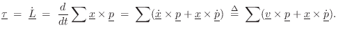
In summary, force equals the time-derivative of linear momentum, and torque equals the time-derivative of angular momentum. By Newton's laws, the time-derivative of linear momentum is mass times acceleration, and the time-derivative of angular momentum is the mass moment of inertia times angular acceleration:

$\displaystyle \dot{p_t}=ma_t\;\;\;\Leftrightarrow\;\;\; \dot{L}=I\alpha$

Equations of Motion for Rigid Bodies

We are now ready to write down the general equations of motion for rigid bodies in terms of for the center of mass and $\tau=I\alpha$ for the rotation of the body about its center of mass.

As discussed above, it is useful to decompose the motion of a rigid body into

(1): the linear velocity $\underline{v}$ of its center of mass, and
(2): its angular velocity $\underline{\omega}$ about its center of mass.

The linear motion is governed by Newton's second law $\underline{f}=M\dot{\underline{v}}$ , where is the total mass, $\underline{v}$ is the velocity of the center-of-mass, and $\underline{f}$ is the sum of all external forces on the rigid body. (Equivalently, $\underline{f}$ is the sum of the radial force components pointing toward or away from the center of mass.) Since this is so straightforward, essentially no harder than dealing with a point mass, we will not consider it further.

The angular motion is governed the rotational version of Newton's second law introduced in §B.4.19:

$\displaystyle \underline{\tau}\eqsp \dot{\underline{L}} \eqsp \mathbf{I}\,\dot{\underline{\omega}} \eqsp \mathbf{I}\,\dot{\underline{\omega}} \protect$

(B.29)

where $\tau$ is the vector torque defined in Eq. $\,$ (B.27), $\underline{L}$ is the angular momentum, $\mathbf{I}$ is the mass moment of inertia tensor, and $\underline{\omega}$ is the angular velocity of the rigid body about its center of mass. Note that if the center of mass is moving, we are in a moving coordinate system moving with the center of mass (see next section). We may call $\underline{L}$ the intrinsic momentum of the rigid body, i.e., that in a coordinate system moving with the center of the mass. We will translate this to the non-moving coordinate system in §B.4.20 below.

The driving torque $\underline{\tau}$ is given by the resultant moment of the external forces, using Eq. $\,$ (B.27) for each external force to obtain its contribution to the total moment. In other words, the external moments (tangential forces times moment arms) sum up for the net torque just like the radial force components summed to produce the net driving force on the center of mass.

Body-Fixed and Space-Fixed Frames of Reference

Rotation is always about some (instantaneous) axis of rotation that is free to change over time. It is convenient to express rotations in a coordinate system having its origin ( $\underline{0}$ ) located at the center-of-mass of the rigid body (§B.4.1), and its coordinate axes aligned along the principal directions for the body (§B.4.16). This body-fixed frame then moves within a stationary space-fixed frame (or ``star frame'').

In Eq. $\,$ (B.29) above, we wrote down Newton's second law for angular motion in the body-fixed frame, i.e., the coordinate system having its origin at the center of mass. Furthermore, it is simplest ( $\mathbf{I}$ is diagonal) when its axes lie along principal directions (§B.4.16).

As an example of a local body-fixed coordinate system, consider a spinning top. In the body-fixed frame, the ``vertical'' axis coincides with the top's axis of rotation (spin). As the top loses rotational kinetic energy due to friction, the top's rotation-axis precesses around a circle, as observed in the space-fixed frame. The other two body-fixed axes can be chosen as any two mutually orthogonal axes intersecting each other (and the spin axis) at the center of mass, and lying in the plane orthogonal to the spin axis. The space-fixed frame is of course that of the outside observer's inertial frame^B.28in which the top is spinning.

Angular Motion in the Space-Fixed Frame

Let's now consider angular motion in the presence of linear motion of the center of mass. In general, we have [270]

$\displaystyle \underline{L}\eqsp \sum \underline{x}\times \underline{p}$

where the sum is over all mass particles in the rigid body, and $\underline{p}$ denotes the vector linear momentum for each particle. That is, the angular momentum is given by the tangential component of the linear momentum times the associated moment arm. Using the chain rule for differentiation, we find

$\displaystyle \underline{\tau}\eqsp \dot{\underline{L}} \eqsp \frac{d}{dt}\sum ... ...m (\underline{v}\times\underline{p}+ \underline{x}\times \dot{\underline{p}}).$

However, $\underline{v}\times \underline{p}=\underline{v}\times m\underline{v}=\underline{0}$ , so that

$\displaystyle \underline{\tau}\eqsp \dot{\underline{L}} \eqsp \sum \underline{x}\times \dot{\underline{p}} \eqsp \sum \underline{x}\times \underline{f}$

which is the sum of moments of all external forces.

Euler's Equations for Rotations in the Body-Fixed Frame

Suppose now that the body-fixed frame is rotating in the space-fixed frame with angular velocity $\underline{\omega}$ . Then the total torque on the rigid body becomes [270]

$\displaystyle \underline{\tau}\eqsp \dot{\underline{L}} + \underline{\omega}\times \underline{L}. \protect$

(B.30)

Similarly, the total external forces on the center of mass become

$\displaystyle \underline{f}\eqsp \dot{\underline{p}} + \underline{\omega}\times\underline{p}.$

If the body-fixed frame is aligned with the principal axes of rotation (§B.4.16), then the mass moment of inertia tensor is diagonal, say $\mathbf{I}=$ diag

. In this frame, the angular momentum is simply

$\displaystyle \underline{L}\eqsp \left[\begin{array}{c} I_1\omega_1 \\ [2pt] I_2\omega_2 \\ [2pt] I_3\omega_3\end{array}\right]$

so that the term $\underline{\omega}\times\underline{L}$ becomes (cf. Eq. $\,$ (B.15))

$\begin{eqnarray*} \underline{\omega}\times\underline{L}&=& \left\vert \begin{arr... ...1\,\underline{e}_2 + (I_2-I_1)\omega_1\omega_2\,\underline{e}_3. \end{eqnarray*}$

Substituting this result into Eq. $\,$ (B.30), we obtain the following equations of angular motion for an object rotating in the body-fixed frame defined by its three principal axes of rotation:

$\begin{eqnarray*} \tau_1 &=& I_1 \dot{\omega}_1 + (I_3-I_2)\omega_2\omega_3\\ \... ...a_1\\ \tau_3 &=& I_3 \dot{\omega}_3 + (I_2-I_1)\omega_1\omega_2 \end{eqnarray*}$

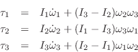
These are call Euler's equations:^B.29Since these equations are in the body-fixed frame, is the mass moment of inertia about principal axis , and $\omega_i$ is the angular velocity about principal axis .

Examples

For a uniform sphere, the cross-terms disappear and the moments of inertia are all the same, leaving $\tau_i=I\omega_i$ , for . Since any three orthogonal vectors can serve as eigenvectors of the moment of inertia tensor, we have that, for a uniform sphere, any three orthogonal axes can be chosen as principal axes.

For a cylinder that is not spinning about its axis, we similarly obtain two uncoupled equations $\tau_i=I\omega_i$ , for , given $\omega_3=\tau_3=0$ (no spin). Note, however, that if we replace the circular cross-section of the cylinder by an ellipse, then $I_1\ne I_2$ and there is a coupling term that drives $\dot{\omega}_3$ (unless $\tau_3$ happens to cancel it).

Next Section:
Properties of Elastic Solids
Previous Section:
Momentum