


Gaussian Function Properties
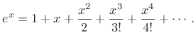
This appendix collects together various facts about the fascinating Gaussian function--the classic ``bell curve'' that arises repeatedly in science and mathematics. As already seen in §B.17.1, only the Gaussian achieves the minimum time-bandwidth product among all smooth (analytic) functions.
Gaussian Window and Transform
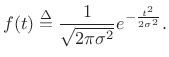
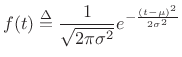
The Gaussian window for FFT analysis was introduced in §3.11, and complex Gaussians (``chirplets'') were utilized in §10.6. For reference in support of these topics, this appendix derives some additional properties of the Gaussian, defined by
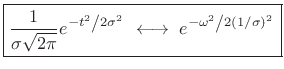 |
(D.1) |
and discusses some interesting applications in spectral modeling (the subject of §10.4). The basic mathematics rederived here are well known (see, e.g., [202,5]), while the application to spectral modeling of sound remains a topic under development.
Gaussians Closed under Multiplication
Define
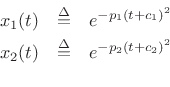
where
![]() are arbitrary complex numbers. Then by direct
calculation, we have
are arbitrary complex numbers. Then by direct
calculation, we have
![\begin{eqnarray*}
x_1(t)\cdot x_2(t)
&=& e^{-p_1(t+c_1)^2} e^{-p_2(t+c_2)^2}\\
&=& e^{-p_1 t^2 - 2 p_1 c_1 t - p_1 c_1^2 -p_2 t^2 - 2 p_2 c_2 t - p_2 c_2^2}\\
&=& e^{-(p_1+p_2) t^2 - 2 (p_1 c_1 + p_2 c_2) t - (p_1 c_1^2 + p_2 c_2^2)}\\
&=& e^{-(p_1+p_2)\left[t^2 + 2\frac{p_1 c_1 + p_2 c_2}{p_1 + p_2} t
+ \frac{p_1 c_1^2 + p_2 c_2^2}{p_1 + p_2}\right]}
\end{eqnarray*}](http://www.dsprelated.com/josimages_new/sasp2/img2726.png)
Completing the square, we obtain
| (D.2) |
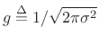
with
![\begin{eqnarray*}
p &=& p_1+p_2\\ [5pt]
c &=& \frac{p_1 c_1 + p_2 c_2}{p_1 + p_2}\\ [5pt]
g &=& e^{-p_1 p_2 \frac{(c_1 - c_2)^2}{p_1 + p_2}}
\end{eqnarray*}](http://www.dsprelated.com/josimages_new/sasp2/img2728.png)
Note that this result holds for Gaussian-windowed chirps
(![]() and
and ![]() complex).
complex).
Product of Two Gaussian PDFs
For the special case of two Gaussian probability densities,
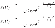
the product density has mean and variance given by
![\begin{eqnarray*}
\mu &=&
\frac{\frac{\mu_1}{2\sigma_1^2} + \frac{\mu_2}{2\sigma_2^2}}{\frac{1}{2\sigma_1^2} + \frac{1}{2\sigma_2^2}}
\;\eqsp \;
\frac{\mu_1\sigma_2^2 + \mu_2\sigma_1^2}{\sigma_2^2 + \sigma_1^2}\\ [5pt]
\sigma^2 &=& \left. \sigma_1^2 \right\Vert \sigma_2^2 \;\isdefs \;
\frac{1}{\frac{1}{\sigma_1^2} + \frac{1}{\sigma_2^2}} \;\eqsp \;
\frac{\sigma_1^2\sigma_2^2}{\sigma_1^2 + \sigma_2^2}.
\end{eqnarray*}](http://www.dsprelated.com/josimages_new/sasp2/img2730.png)
Gaussians Closed under Convolution
In §D.8 we show that
- the Fourier transform of a Gaussian is Gaussian, and in §D.2 that
- the product of any two Gaussians is Gaussian.
Fitting a Gaussian to Data
When fitting a single Gaussian to data, one can take a log and fit a parabola. In matlab, this can be carried out as in the following example:
x = -1:0.1:1;
sigma = 0.01;
y = exp(-x.*x) + sigma*randn(size(x)); % test data:
[p,s] = polyfit(x,log(y),2); % fit parabola to log
yh = exp(polyval(p,x)); % data model
norm(y-yh) % ans =  1.9230e-16 when sigma=0
plot(abs([y',yh']));
In practice, it is good to avoid zeros in the data. For example, one can fit only to the middle third or so of a measured peak, restricting consideration to measured samples that are positive and ``look Gaussian'' to a reasonable extent.
Infinite Flatness at Infinity
The Gaussian is infinitely flat at infinity. Equivalently, the
Maclaurin expansion (Taylor expansion about ![]() ) of
) of
| (D.3) |
is zero for all orders. Thus, even though
 |
(D.4) |
for all
 |
(D.5) |
We may call
- Padé approximation is maximally flat approximation, and seeks
to use all
 degrees of freedom in the approximation to match
the
leading terms of the Taylor series expansion.
degrees of freedom in the approximation to match
the
leading terms of the Taylor series expansion.
- Butterworth filters (IIR) are maximally flat at dc [263].
- Lagrange interpolation (FIR) is maximally flat at dc [266].
- Thiran allpass interpolation has maximally flat group delay at dc [266].
Another interesting mathematical property of essential singularities is
that near an essential singular point
![]() the
inequality
the
inequality
| (D.6) |
is satisfied at some point
Integral of a Complex Gaussian
Theorem:
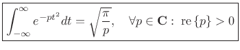 |
(D.7) |
Proof: Let ![]() denote the integral. Then
denote the integral. Then
where we needed
re![]() to have
to have
![]() as
as
![]() . Thus,
. Thus,
 |
(D.8) |
as claimed.
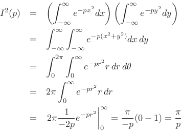
Area Under a Real Gaussian
Corollary:
Setting
![]() in the previous theorem, where
in the previous theorem, where ![]() is real,
we have
is real,
we have
 |
(D.9) |
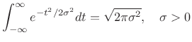
Therefore, we may normalize the Gaussian to unit area by defining
 |
(D.10) |
Since
 |
(D.11) |
it satisfies the requirements of a probability density function.
Gaussian Integral with Complex Offset
Theorem:
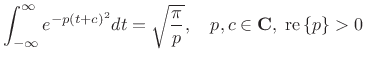 |
(D.12) |
Proof:
When ![]() , we have the previously proved case. For arbitrary
, we have the previously proved case. For arbitrary
![]() and real number
and real number
![]() , let
, let
![]() denote the closed rectangular contour
denote the closed rectangular contour
![]() , depicted in Fig.D.1.
, depicted in Fig.D.1.
![\includegraphics[width=0.8\twidth]{eps/gammarect}](http://www.dsprelated.com/josimages_new/sasp2/img2762.png)
Clearly,
 is analytic inside the region bounded
by
is analytic inside the region bounded
by
![]() . By Cauchy's theorem [42],
the line integral of
. By Cauchy's theorem [42],
the line integral of ![]() along
along
![]() is zero, i.e.,
is zero, i.e.,
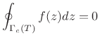 |
(D.13) |
This line integral breaks into the following four pieces:
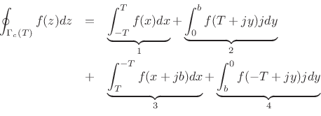
where ![]() and
and ![]() are real variables. In the limit as
are real variables. In the limit as
![]() ,
the first piece approaches
,
the first piece approaches
![]() , as previously proved.
Pieces
, as previously proved.
Pieces ![]() and
and ![]() contribute zero in the limit, since
contribute zero in the limit, since
![]() as
as
![]() . Since the total contour integral is
zero by Cauchy's theorem, we conclude that piece 3 is the negative of
piece 1, i.e., in the limit as
. Since the total contour integral is
zero by Cauchy's theorem, we conclude that piece 3 is the negative of
piece 1, i.e., in the limit as
![]() ,
,
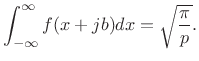 |
(D.14) |
Making the change of variable
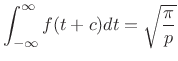 |
(D.15) |
as desired.
Fourier Transform of Complex Gaussian
Theorem:
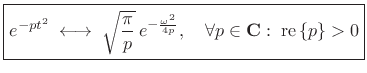 |
(D.16) |
Proof: [202, p. 211]
The Fourier transform of ![]() is defined as
is defined as
 |
(D.17) |
Completing the square of the exponent gives
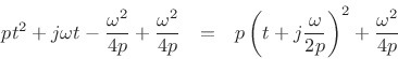
Thus, the Fourier transform can be written as
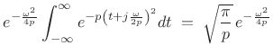 |
(D.18) |
using our previous result.
Alternate Proof
The Fourier transform of a complex Gaussian can also be derived using the differentiation theorem and its dual (§B.2).D.1
Proof: Let
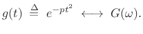 |
(D.19) |
Then by the differentiation theorem (§B.2),
| (D.20) |
By the differentiation theorem dual (§B.3),
| (D.21) |
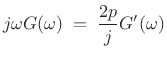
Differentiating
![$\displaystyle g^\prime(t) \eqsp -2ptg(t) \eqsp \frac{2p}{j}[-jtg(t)] \;\longleftrightarrow\;\frac{2p}{j}G^\prime(\omega).$](http://www.dsprelated.com/josimages_new/sasp2/img2780.png) |
(D.22) |
Therefore,
 |
(D.23) |
or
![$\displaystyle \left[\ln G(\omega)\right]^\prime \eqsp \frac{G^\prime(\omega)}{G(\omega)} \eqsp -\frac{\omega}{2p} \eqsp \left(-\frac{\omega^2}{4p}\right)^\prime.$](http://www.dsprelated.com/josimages_new/sasp2/img2782.png) |
(D.24) |
Integrating both sides with respect to
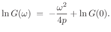 |
(D.25) |
In §D.7, we found that
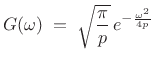 |
(D.26) |
as expected.
The Fourier transform of complex Gaussians (``chirplets'') is used in §10.6 to analyze Gaussian-windowed ``chirps'' in the frequency domain.
Why Gaussian?
This section lists some of the points of origin for the Gaussian function in mathematics and physics.
Central Limit Theorem
The central limit theoremD.2provides that many iterated convolutions of any ``sufficiently regular'' shape will approach a Gaussian function.
Iterated Convolutions
Any ``reasonable'' probability density function (PDF) (§C.1.3)
has a Fourier transform that looks like
![]() near its tip. Iterating
near its tip. Iterating ![]() convolutions then corresponds to
convolutions then corresponds to
![]() , which becomes
[2]
, which becomes
[2]
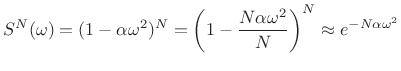 |
(D.27) |
for large
Since the inverse Fourier transform of a Gaussian is another Gaussian
(§D.8), we can define a time-domain function ![]() as
being ``sufficiently regular'' when its Fourier transform approaches
as
being ``sufficiently regular'' when its Fourier transform approaches
![]() in a sufficiently small
neighborhood of
in a sufficiently small
neighborhood of ![]() . That is, the Fourier transform simply
needs a ``sufficiently smooth peak'' at
. That is, the Fourier transform simply
needs a ``sufficiently smooth peak'' at ![]() that can be
expanded into a convergent Taylor series. This obviously holds for
the DTFT of any discrete-time window function
that can be
expanded into a convergent Taylor series. This obviously holds for
the DTFT of any discrete-time window function ![]() (the subject of
Chapter 3), because the window transform
(the subject of
Chapter 3), because the window transform ![]() is a finite
sum of continuous cosines of the form
is a finite
sum of continuous cosines of the form
![]() in the
zero-phase case, and complex exponentials in the causal case, each of
which is differentiable any number of times in
in the
zero-phase case, and complex exponentials in the causal case, each of
which is differentiable any number of times in ![]() .
.
Binomial Distribution
The last row of Pascal's triangle (the binomial distribution) approaches a sampled Gaussian function as the number of rows increases.D.3 Since Lagrange interpolation (elementary polynomial interpolation) is equal to binomially windowed sinc interpolation [301,134], it follows that Lagrange interpolation approaches Gaussian-windowed sinc interpolation at high orders.
Gaussian Probability Density Function
Any non-negative function which integrates to 1 (unit total area) is suitable for use as a probability density function (PDF) (§C.1.3). The most general Gaussian PDF is given by shifts of the normalized Gaussian:
 |
(D.28) |
The parameter
Maximum Entropy Property of the
Gaussian Distribution
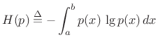
Entropy of a Probability Distribution
The entropy of a probability density function (PDF) ![]() is
defined as [48]
is
defined as [48]
![$\displaystyle \zbox {h(p) \isdef \int_x p(x) \cdot \lg\left[\frac{1}{p(x)}\right] dx}$](http://www.dsprelated.com/josimages_new/sasp2/img2794.png) |
(D.29) |
where
![$\displaystyle h(p) = {\cal E}_p\left\{\lg \left[\frac{1}{p(x)}\right]\right\}$](http://www.dsprelated.com/josimages_new/sasp2/img2796.png) |
(D.30) |
The term
Example: Random Bit String
Consider a random sequence of 1s and 0s, i.e., the probability of a 0 or
1 is always
![]() . The corresponding probability density function
is
. The corresponding probability density function
is
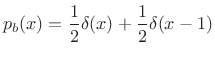 |
(D.31) |
and the entropy is
 |
(D.32) |
Thus, 1 bit is required for each bit of the sequence. In other words, the sequence cannot be compressed. There is no redundancy.
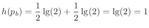
If instead the probability of a 0 is 1/4 and that of a 1 is 3/4, we get
and the sequence can be compressed about ![]() .
.
In the degenerate case for which the probability of a 0 is 0 and that of a 1 is 1, we get
![\begin{eqnarray*}
p_b(x) &=& \lim_{\epsilon \to0}\left[\epsilon \delta(x) + (1-\epsilon )\delta(x-1)\right]\\
h(p_b) &=& \lim_{\epsilon \to0}\epsilon \cdot\lg\left(\frac{1}{\epsilon }\right) + 1\cdot\lg(1) = 0.
\end{eqnarray*}](http://www.dsprelated.com/josimages_new/sasp2/img2803.png)
Thus, the entropy is 0 when the sequence is perfectly predictable.
Maximum Entropy Distributions
Uniform Distribution
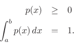
Among probability distributions ![]() which are nonzero over a
finite range of values
which are nonzero over a
finite range of values ![]() , the maximum-entropy
distribution is the uniform distribution. To show this, we
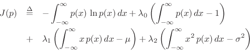
must maximize the entropy,
, the maximum-entropy
distribution is the uniform distribution. To show this, we
must maximize the entropy,
 |
(D.33) |
with respect to
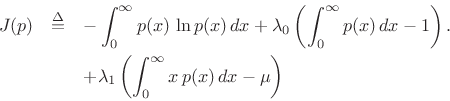
Using the method of Lagrange multipliers for optimization in the presence of constraints [86], we may form the objective function
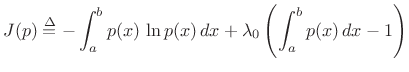 |
(D.34) |
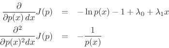
and differentiate with respect to
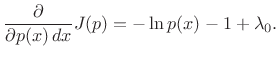 |
(D.35) |
Setting this to zero and solving for
| (D.36) |
(Setting the partial derivative with respect to
Choosing ![]() to satisfy the constraint gives
to satisfy the constraint gives
![]() , yielding
, yielding
![$\displaystyle p(x) = \left\{\begin{array}{ll} \frac{1}{b-a}, & a\leq x \leq b \\ [5pt] 0, & \hbox{otherwise}. \\ \end{array} \right.$](http://www.dsprelated.com/josimages_new/sasp2/img2812.png) |
(D.37) |
That this solution is a maximum rather than a minimum or inflection point can be verified by ensuring the sign of the second partial derivative is negative for all
 |
(D.38) |
Since the solution spontaneously satisfied
Exponential Distribution
Among probability distributions ![]() which are nonzero over a
semi-infinite range of values
which are nonzero over a
semi-infinite range of values
![]() and having a finite
mean
and having a finite
mean ![]() , the exponential distribution has maximum entropy.
, the exponential distribution has maximum entropy.
To the previous case, we add the new constraint
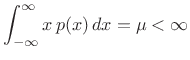 |
(D.39) |
resulting in the objective function
Now the partials with respect to ![]() are
are
and ![]() is of the form
is of the form
![]() . The
unit-area and finite-mean constraints result in
. The
unit-area and finite-mean constraints result in
![]() and
and
![]() , yielding
, yielding
![$\displaystyle p(x) = \left\{\begin{array}{ll} \frac{1}{\mu} e^{-x/\mu}, & x\geq 0 \\ [5pt] 0, & \hbox{otherwise}. \\ \end{array} \right.$](http://www.dsprelated.com/josimages_new/sasp2/img2822.png) |
(D.40) |
Gaussian Distribution
The Gaussian distribution has maximum entropy relative to all
probability distributions covering the entire real line
![]() but having a finite mean
but having a finite mean ![]() and finite
variance
and finite
variance ![]() .
.
Proceeding as before, we obtain the objective function
and partial derivatives
leading to
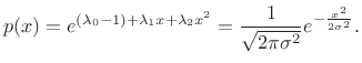 |
(D.41) |
For more on entropy and maximum-entropy distributions, see [48].
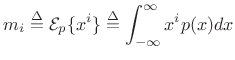
Gaussian Moments
Gaussian Mean
The mean of a distribution ![]() is defined as its
first-order moment:
is defined as its
first-order moment:
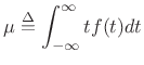 |
(D.42) |
To show that the mean of the Gaussian distribution is ![]() , we may write,
letting
, we may write,
letting
 ,
,
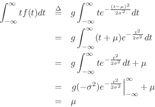
since
![]() .
.
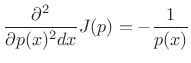
Gaussian Variance
The
variance of a distribution
![]() is defined as its
second central moment:
is defined as its
second central moment:
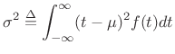 |
(D.43) |
where
To show that the variance of the Gaussian distribution is ![]() , we write,
letting
,
, we write,
letting
,
where we used integration by parts and the fact that
![]() as
as
![]() .
.
Higher Order Moments Revisited
Theorem:
The ![]() th central moment of the Gaussian pdf
th central moment of the Gaussian pdf ![]() with mean
with mean ![]() and variance
and variance ![]() is given by
is given by
![$\displaystyle m_n \isdef {\cal E}_p\{(x-\mu)^n\} = \left\{\begin{array}{ll} (n-1)!!\cdot\sigma^n, & \hbox{$n$\ even} \\ [5pt] $0$, & \hbox{$n$\ odd} \\ \end{array} \right. \protect$](http://www.dsprelated.com/josimages_new/sasp2/img2834.png)
where
Proof:
The formula can be derived by successively differentiating the
moment-generating function
![]() with respect to
with respect to ![]() and evaluating at
and evaluating at ![]() ,D.4 or by differentiating the
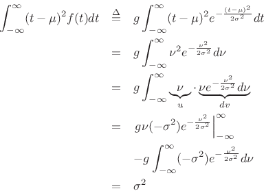
Gaussian integral
,D.4 or by differentiating the
Gaussian integral
 |
(D.45) |
successively with respect to
![\begin{eqnarray*}
\int_{-\infty}^\infty (-x^2) e^{-\alpha x^2} dx &=& \sqrt{\pi}(-1/2)\alpha^{-3/2}\\
\int_{-\infty}^\infty (-x^2)(-x^2) e^{-\alpha x^2} + dx &=& \sqrt{\pi}(-1/2)(-3/2)\alpha^{-5/2}\\
\vdots & & \vdots\\
\int_{-\infty}^\infty x^{2k} e^{-\alpha x^2} dx &=& \sqrt{\pi}\,[(2k-1)!!]\,2^{-k/2}\alpha^{-(k+1)/2}
\end{eqnarray*}](http://www.dsprelated.com/josimages_new/sasp2/img2843.png)
for
![]() .
Setting
.
Setting
![]() and
and ![]() , and dividing both sides by
, and dividing both sides by
![]() yields
yields
 |
(D.46) |
for
Moment Theorem
Theorem:
For a random variable ![]() ,
,
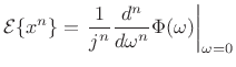 |
(D.47) |
where
 |
(D.48) |
(Note that
Proof: [201, p. 157]
Let ![]() denote the
denote the ![]() th moment of
th moment of ![]() , i.e.,
, i.e.,
 |
(D.49) |
Then
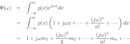
where the term-by-term integration is valid when all moments ![]() are
finite.
are
finite.
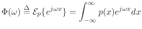
Gaussian Characteristic Function
Since the Gaussian PDF is
 |
(D.50) |
and since the Fourier transform of
| (D.51) |
It follows that the Gaussian characteristic function is
| (D.52) |
Gaussian Central Moments
The characteristic function of a zero-mean Gaussian is
| (D.53) |
Since a zero-mean Gaussian
 |
(D.54) |
In particular,
![\begin{eqnarray*}
\Phi^\prime(\omega) &=& -\frac{1}{2}\sigma^2 2\omega\Phi(\omega)\\ [5pt]
\Phi^{\prime\prime}(\omega) &=& -\frac{1}{2}\sigma^2 2\omega\Phi^\prime(\omega)
-\frac{1}{2}\sigma^2 2\Phi(\omega)
\end{eqnarray*}](http://www.dsprelated.com/josimages_new/sasp2/img2865.png)
Since ![]() and
and
![]() , we see
, we see ![]() ,
,
![]() , as expected.
, as expected.
A Sum of Gaussian Random Variables is a Gaussian Random Variable
A basic result from the theory of random variables is that when you sum two independent random variables, you convolve their probability density functions (PDF). (Equivalently, in the frequency domain, their characteristic functions multiply.)
That the sum of two independent Gaussian random variables is Gaussian follows immediately from the fact that Gaussians are closed under multiplication (or convolution).
Next Section:
Bilinear Frequency-Warping for Audio Spectrum Analysis over Bark and ERB Frequency Scales
Previous Section:
Beginning Statistical Signal Processing


